

2024-10-10
Energy on a closed turn of a coil
This study is somewhat reminiscent of Tesla's experiment with a U-shaped busbar,
but unlike it, here we will consider the energy arising on the transverse closed turn of the toroidal coil.
From classical electrodynamics it is known that the magnetic field vector \(\vec B\) in a toroidal ferrite core,
generated by a current-carrying wire wound on it, will be located along the circumference, and only inside the core (Fig. 1a).
In this study, we will show that for sufficiently short pulses on the generating winding, another field appears in the core, perpendicular to the classical vortex field,
we will light an LED from it, located on a closed turn of the conductor, and draw conclusions about some properties of this field.

Fig. 1. Here: a - diagram of the magnetic field \(\vec B\) in the toroidal core, b - experiment diagram,
c - connection of the LED D1 to the copper tape W2 (a cross-section of the core A-A is shown)
|
To conduct our study, we will need a toroidal ferromagnetic core F1 (Fig. 1b).
The author used three ferrite rings folded together as such a core, each measuring 124*78*12 mm, and a relative magnetic permeability of 2000 units.
Transformer T1 is made from them as follows.
A wire in insulation is wound on one side of the core, 4-6 turns, forming a transmitting winding W1, to which the pulse generator GG1 is connected.
The author used such a generator, but any other similar one with a good pulse rise and fall time will do for these experiments.
At 90 degrees from W1, the core is covered with an uninsulated turn of copper tape, closed and sealed in this place.
This turn will be the receiving coil W2.
It should be noted that W2 can also be placed on the opposite side of the core from W1, but the effect will be slightly worse.
The most important moment here is the connection of the LED D1.
In the end, it should light up on a completely closed turn, which in itself will be a unique non-classical effect.
To do this, its terminals should be soldered to the copper tape so that the soldering points are located as far from each other as possible (Fig. 1c).
With this connection, the brightness of the LED will be maximum. But, as in Tesla's experiment, it will also light up in other places where it is connected to the tape.
A photo of a glowing LED connected in this way can be seen in Figures 2 and 3.
In these studies, the author used a LED with a power of 3 W.
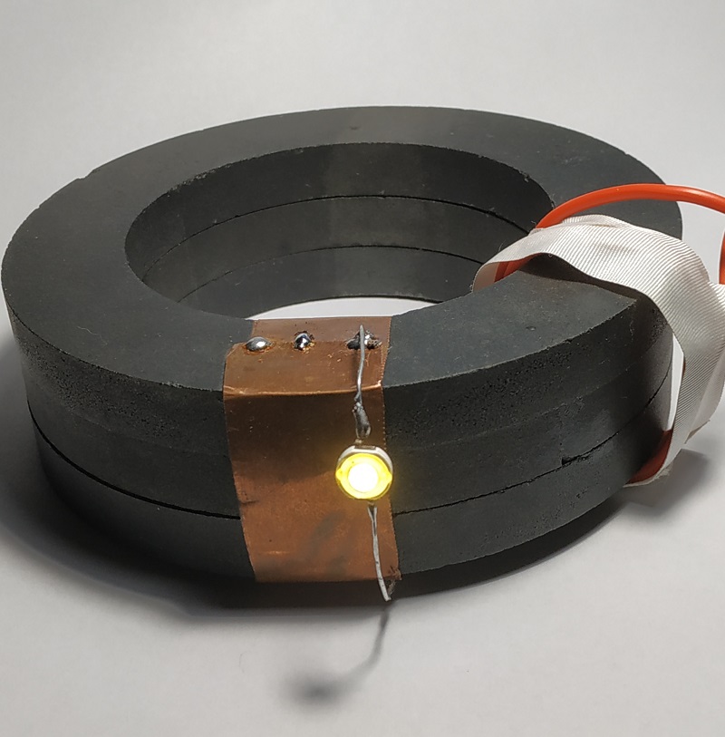
Fig. 2. Glow of D1 in a transverse magnetic field | 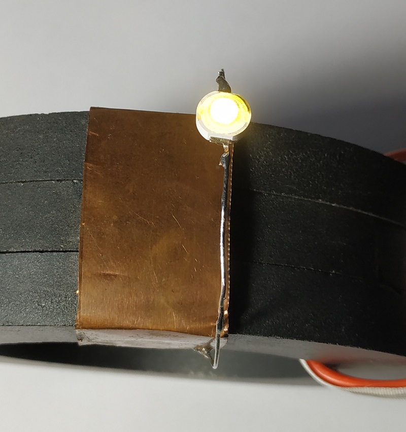 Fig.3. The same inclusion, bottom view | 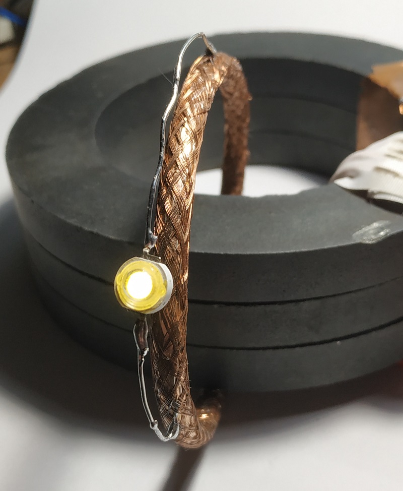 Fig.4. Glow of D1 on a closed loop
|
It should be noted that the efficiency of such a circuit is quite low, and its meaning is to demonstrate a field, albeit weak, that completely contradicts the official electrodynamics.
To fix this effect, you can also make a closed loop of copper wire instead of a tape (the author used a piece of coaxial cable without braiding).
If you connect an LED to it, it will also glow (Fig. 4).
It is interesting that connecting the load in this way does not affect the current consumption of the generator, which was measured with precision instruments.
Parameters of the GG1 generator.
The pulse repetition rate is 70.3 kHz, which is not a constant. The frequency can, in principle, be any.
The power supplied to the GG1 generator was approximately 1 W, and the voltage was 20 V, which is also not an absolute value.
It is important that the pulse shape is approximately the same as in Figure 7 (blue beam).
In the declared generator this is achieved by adjusting the pulse duration with resistor R1.
In order to clearly understand that this is a different type of field, possessing a different classsic vortex field regularity, the author connected the OS1 oscilloscope instead of the LED.
But the first oscillogram (Fig. 5) shows pulses on the W1 coil, measured directly on it with a high-voltage probe.
The second oscillogram is located in Figure 6.
To measure the current flowing through W1, the circuit, along the positive supply, was connected through a low-resistance resistance of 0.9 Ohm.
The yellow beam probe was connected to this resistance. We will use this current in the following oscillograms.
The blue beam probe is connected to a turn of wire put on the core in order to check the voltage pulse on the classic secondary winding.
As we can see, the shape of this voltage pulse is almost no different from the shape of the current pulse, and therefore the magnetic field in the F1 core (Fig. 1b).
The third oscillogram is shown in Figure 7.
Further measurements with a probe directly on the W1 coil greatly blurred the picture of the processes occurring in the circuit, so the probe (blue beam) was connected through the insulator to the wire from the GG1 generator.
The other probe (yellow beam) shows the current through W1.
As we can see, the shape of the voltage pulse is almost the same as the shape of the current pulse, and therefore the magnetic field in the F1 core (Fig. 1b).
By the way, this state of affairs occurs during resonance of the second kind.
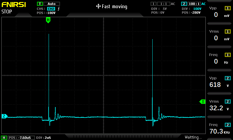 Fig.5. Voltage pulses on coil W1 | 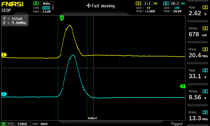 Fig.6. Voltage pulse on a turn of wire (blue beam), and current through W1 (yellow beam) |  Fig.7. Voltage pulse on W1 (blue beam), and current through W1 (yellow beam)
|
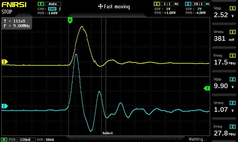
Fig. 8. Current pulse through W1 (yellow beam), and voltage on the W2 coil without LED (blue beam)
|
Particular attention should be paid to the fourth oscillogram (Fig. 8).
It shows the already known current pulse through W1, measured on a low-resistance resistor (yellow beam), which determines the magnetic field \(B\) in the core,
and the reaction to a change of this field in the receiving coil W2, measured with the LED turned off (blue beam).
The following pattern can be traced here:
\[ U_2 \sim {d B \over d t} \sim {d U_1 \over d t} \tag{1}\]
where \(U_1\) is the amplitude of the signal on the coil W1, \(U_2\) is the amplitude of the signal on the coil W2, and \(t\) is time.
In other words, the signal on the receiving coil is proportional to the change in the vortex magnetic field in the core.
Also, the signal on W2 is proportional to the change in voltage on W1.
For comparison, it should be said that in a classic unloaded transformer, the pattern (1) would look like this:
\[ U_2 \sim U_1 \tag{2}\]
That is, the voltage on the receiving coil W2 would be proportional to the voltage on the transmitting coil W1.

Fig. 9. Output key of the GG1 generator with capacitor C1
|
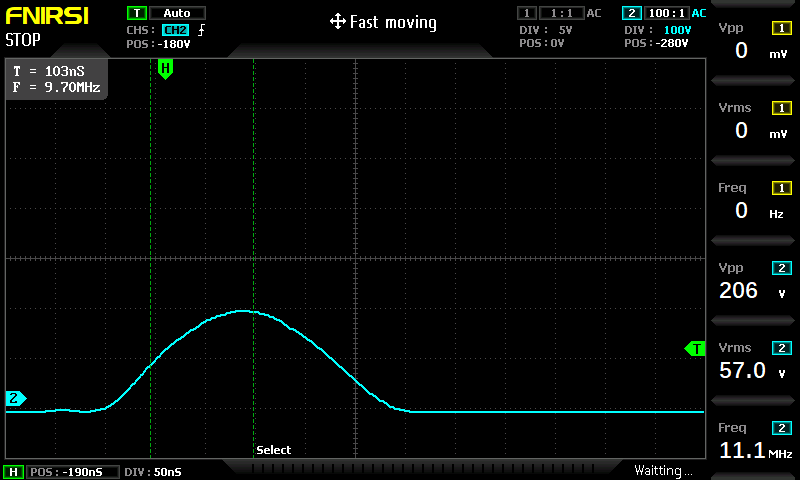
Fig. 10. Oscillogram of a pulse on W1 with capacitor C1
|
Another fact confirming that the voltage on W2 changes according to the law of expression (1)
can be the connection of an additional capacitor C1 in parallel with the output key in GG1 (Fig. 9).
With an additional 200 pF, the brightness of D1 drops sharply, and with a capacitance of 1000 pF, the LED stops glowing and the effect disappears.
At the same time, the pulse duration on W1 changes from 60 ns to 250 ns, but the pulse area (Fig. 10) and the generator power consumption do not change.
That is, with an increase in the rise and fall time of the master pulse, with the same energy pumped into the core, the "transverse" energy decreases inversely proportionally.
Conclusions
Thanks to this effect, we were able to light the LED, which is connected to a closedmu turn, covering the ferromagnetic core.
But if the front and fall of the master pulse have a greater flatness, then even with the same transmitted power from the generator, the LED reduces the brightness of its glow down to zero.
The parameters of the front and rise of the master pulse play a decisive role here.
Hence, an obvious way to increase the efficiency of this method of energy transfer follows, which consists in improving the parameters of the master pulse and the frequency properties of the ferromagnetic core.
Based on the data obtained, it can be assumed that the declared "transverse" energy is formed due to the
second magnetic (scalar) field.
Such a field appears when the vortex magnetic field changes according to law (1) and perpendicular to it in the direction of the magnetic lines of force.