

2026-08-31
Acceleration as a projection of uniform motion of higher splittings
Why Acceleration is an Illusion
Imagine you're speeding in a car and suddenly you slam on the brakes. The tires squeal, the road hums, the belt tugs, and you're thrown forward with all your might. It seems as if nothing could be more real than this acceleration. But what if the sensation itself is quite real, and the acceleration isn't fundamental? What if the world we see shows only one projection of a much more complex motion, distributed among many hidden splits? Then, at our level, there's a sudden deceleration, while in the full space of higher levels, none of this occurs: there, a single, uniform, linear motion is preserved. Perhaps acceleration isn't a change in motion per se, but the price we pay for seeing only a small part of the geometry of reality.
Acceleration is usually viewed as a direct change in the particle's motion. If the velocity changes, we say that a force acts on the particle. However, this interpretation ignores the possibility that the observed space is merely a projection of a more complete geometry. In this case, the second derivative of the observed coordinate may be nonzero even when the overall motion remains rectilinear and uniform.
The central idea of this paper is that acceleration is not necessarily a property of the overall motion. It can arise when projecting the uniform motion of the space of higher splittings onto the level accessible to us.
First, let's consider a simple finite-dimensional example in which this mechanism is directly visible. We will then move on to multilevel idempotent splitting and show that an arbitrary smooth subliminal motion can be obtained with arbitrarily high precision from a finite number of uniform higher phases, and precisely in the limit of infinite splitting.
By the way, a similar example is also considered in vector theory, which yields roughly the same results.
1. Two points in a two-dimensional world
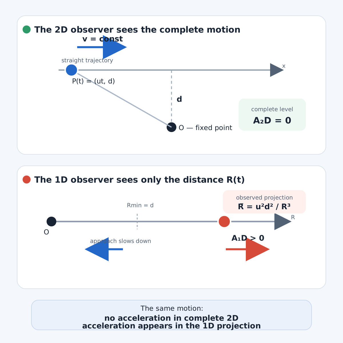 Fig. 1 Acceleration depending on the observer's dimension |
Let the first point be stationary and located at the origin, and the second move uniformly in two-dimensional space:
\[\tag{1} O=(0,0), \qquad P(t)=(ut,d), \] where \(u\) is the constant velocity, and \(d\) is the minimum distance from the stationary point to the trajectory. The velocity vector of the second point is constant:
\[\tag{2} \mathbf v_{2D}=\frac{dP}{dt}=(u,0)=\operatorname{const}. \] Therefore, its total two-dimensional acceleration is zero:
\[\tag{3} \boxed{ \mathbf A_{2D}=\frac{d\mathbf v_{2D}}{dt}=0. } \] Now imagine a one-dimensional observer whose only axis always passes between two points. He does not see the coordinates \(x\) and \(y\) separately. His only observable coordinate is the distance between the points:
\[\tag{4} R(t)=\sqrt{d^2+u^2t^2}. \] One-dimensional velocity is
\[\tag{5} \dot R(t)=\frac{u^2t}{\sqrt{d^2+u^2t^2}}=\frac{u^2t}{R}. \] It changes over time. Further differentiation yields
\[\tag{6} \boxed{ \ddot R(t)=\frac{u^2d^2}{\left(d^2+u^2t^2\right)^{3/2}} =\frac{u^2d^2}{R^3}. } \] Thus, the same motion has two different descriptions:
\[\tag{7} \boxed{ \mathbf A_{2D}=0, \qquad A_{1D}=\ddot R\ne0. } \] At the moment of closest approach (t=0), the one-dimensional velocity is zero, but the acceleration remains nonzero:
\[\tag{8} R(0)=d, \qquad \dot R(0)=0, \qquad \boxed{\ddot R(0)=\frac{u^2}{d}}. \] For a one-dimensional inhabitant, this acceleration is completely natural. The point he observes first approaches more and more slowly, then stops at a distance of \(d\), after which it recedes with ever-increasing speed. He is unaware that his single axis is rotating in a higher-level space.
2. The Hidden Coordinate Compensating for Acceleration
Let's rewrite the same two-dimensional motion in polar coordinates. The full acceleration vector is
\[\tag{9} \mathbf A= \left(\ddot R-R\dot\theta^2\right)\mathbf e_R + \left(R\ddot\theta+2\dot R\dot\theta\right)\mathbf e_\theta. \] But the initial motion is rectilinear and uniform, so \(\mathbf A=0\). In particular, the radial component satisfies the equality
\[\tag{10} \boxed{ \ddot R=R\dot\theta^2. } \] A one-dimensional observer sees only the first expression \(\ddot R\), but not the hidden angular degree of freedom \(\theta\). At the full level, both sides are included in the same equality:
\[\tag{11} \boxed{ \ddot R-R\dot\theta^2=0. } \] Therefore, the observed one-dimensional acceleration arose not from a change in the total motion, but from the loss of the angular coordinate. When the hidden coordinate returns to the description, the acceleration disappears.
What appears to be acceleration at a lower level may be only one component of uniform rectilinear motion at a higher level.
3. Hypothesis on the Projective Nature of Acceleration
The previous example admits of a more general interpretation. Perhaps the space we observe is also a lower level relative to the space of higher splittings. Then the velocity and acceleration available to us may not be complete characteristics of the motion, but the result of a successive reduction of hidden components.
\[\tag{12} \text{complete uniform motion} \xrightarrow{\;\Pi_N\;} \text{observed accelerated motion}. \] In this article, our three-dimensional space is considered as a single, effectively observable direction. We examine only the scalar quantities \(v(t)\) and \(A(t)\), without separating the acceleration into its spatial components. This simplification allows us to first prove the acceleration mechanism itself, and only then generalize it to 3D directions.
The main hypothesis can be formulated as follows:
\[\tag{13} \boxed{ \begin{gathered} \text{the observed acceleration is a consequence of projection,}\\ \text{and in a full space of sufficiently high splitting}\\ \text{the motion remains rectilinear and uniform.} \end{gathered} } \] 4. Multilevel splitting space
Let N independent commuting hyperbolic units be introduced:
\[\tag{14} \j_r^2=1, \qquad \j_r\j_s=\j_s\j_r, \qquad r,s=1,\ldots,N. \] Each unit creates a pair of complementary idempotents:
\[\tag{15} p_r^+=\frac{1+\j_r}{2}, \qquad p_r^-=\frac{1-\j_r}{2}. \] After \(N\) successive splits, \(2^N\) minimal orthogonal channels arise:
\[\tag{16} \boxed{ E_{\boldsymbol{\sigma}} =2^{-N}\prod_{r=1}^{N} \left(1+\sigma_r\j_r\right), \qquad \sigma_r\in\{+1,-1\}. } \] They satisfy the conditions
\[\tag{17} E_{\boldsymbol{\sigma}}E_{\boldsymbol{\tau}} =\delta_{\boldsymbol{\sigma}\boldsymbol{\tau}} E_{\boldsymbol{\sigma}}, \qquad \sum_{\boldsymbol{\sigma}} E_{\boldsymbol{\sigma}}=1. \] This construction is discussed in detail in the article "Multilevel Idempotent Splitting of Phase Planes". What's important here is that each new level doubles the number of mutually orthogonal channels that remain parts of a single unit.
5. Uniform motion of the highest level
We write the general normalized state of the \(N\)th level as
\[\tag{18} J_N(t)= \sum_{\boldsymbol{\sigma}} E_{\boldsymbol{\sigma}} e^{i\phi_{\boldsymbol{\sigma}}(t)}. \] We will consider the higher-level motion to be uniform if each unrolled phase is a linear function of time:
\[\tag{19} \boxed{ \phi_{\boldsymbol{\sigma}}(t) =\omega_{\boldsymbol{\sigma}}t +\phi_{\boldsymbol{\sigma}0}, \qquad \omega_{\boldsymbol{\sigma}}=\operatorname{const}. } \] In phase space, this motion is in a straight line:
\[\tag{20} \boldsymbol{\phi}(t) =\boldsymbol{\phi}_0 +\boldsymbol{\omega}t, \qquad \boxed{\ddot{\boldsymbol{\phi}}=0}. \] The complex images of individual phases rotate, but in the expanded phase space, all components move at constant velocities. It is in this sense that the highest motion is rectilinear and uniform.
The complete norm of the state remains unitary:
\[\tag{21} \begin{aligned} J_N\overline{J_N} &= \sum_{\boldsymbol{\sigma},\boldsymbol{\tau}} E_{\boldsymbol{\sigma}}E_{\boldsymbol{\tau}} e^{i(\phi_{\boldsymbol{\sigma}}-\phi_{\boldsymbol{\tau}})}\\ &= \sum_{\boldsymbol{\sigma}} E_{\boldsymbol{\sigma}} =1. \end{aligned} \] Higher splittings do not create an additional norm. They reveal the internal structure of the previous unit: the geometry of motion is split, but not its full magnitude.
6. Projection onto the observable parameter of motion
According to the accepted rule of the model, the parameter of external motion is related to the velocity by the following relations
\[\tag{22} b(t)=\frac{\arcsin\beta(t)}{\pi}, \qquad \beta(t)=\frac{v(t)}{c}. \] Back:
\[\tag{23} \boxed{ \beta(t)=\sin\bigl(\pi b(t)\bigr), \qquad v(t)=c\sin\bigl(\pi b(t)\bigr). } \] Let the lower level not see individual higher channels, but receive a single scalar parameter from them:
\[\tag{24} b_N(t)=\mathcal B_N[J_N(t)]. \] For a finite number of channels, the natural linear reduction is
\[\tag{25} \boxed{ b_N(t)=b_0+ \sum_{k=1}^{2^N} \operatorname{Re} \left[ c_k e^{i(\omega_kt+\phi_{k0})} \right]. } \] The complex coefficients \(c_k\) define the geometry of the relationship between the higher channels and the observed level. If we write them in terms of real coefficients, we get
\[\tag{26} b_N(t)=b_0+ \sum_{k=1}^{2^N} \left[ A_k\cos(\omega_kt) +B_k\sin(\omega_kt) \right]. \] All higher frequencies are constant, but their overall projection \(b_N(t)\) is no longer constant in the general case.
7. The occurrence of the observed acceleration
The observed velocity at the (Nth)th approximation level is
\[\tag{27} v_N(t)=c\sin\bigl(\pi b_N(t)\bigr). \] Differentiating, we obtain
\[\tag{28} \boxed{ A_N(t)=\frac{dv_N}{dt} =\pi c\cos\bigl(\pi b_N(t)\bigr)\dot b_N(t). } \] In this case,
\[\tag{29} \dot b_N(t)= \sum_{k=1}^{2^N} \omega_k \left[ -A_k\sin(\omega_kt) +B_k\cos(\omega_kt) \right]. \] Thus, the observed acceleration can be variable, although at the highest level.
\[\tag{30} \dot\phi_k=\omega_k=\operatorname{const}, \qquad \ddot\phi_k=0. \] The acceleration of the lower level arises not from the acceleration of the higher phases, but from a change in their overall projection.
The entire sequence of transformations has the form
\[\tag{31} \boxed{ \begin{gathered} \phi_k(t)=\omega_kt+\phi_{k0} \quad\Longrightarrow\quad b_N(t)=\mathcal B_N[J_N(t)] \quad\Longrightarrow\quad\\ v_N(t)=c\sin(\pi b_N) \quad\Longrightarrow\quad A_N(t)=\pi c\cos(\pi b_N)\dot b_N. \end{gathered} } \] 8. When a Finite Number of Splits Sufficient
If the observed motion parameter is itself a finite sum of harmonics,
\[\tag{32} b(t)=b_0+ \sum_{k=1}^{M} \left[ A_k\cos(\omega_kt) +B_k\sin(\omega_kt) \right], \] then it is sufficient to choose a level \(N\) for which
\[\tag{33} \boxed{2^N\ge M}. \] Each harmonic can be associated with a separate idempotent channel. Then \(b(t)\), \(v(t)\), and \(A(t)\) are reproduced exactly.
\[\tag{34} \boxed{ \begin{gathered} \text{If }b(t)\text{ is a finite trigonometric polynomial,}\\ \text{the corresponding acceleration rises exactly}\\ \text{to a finite number of uniform higher phases.} \end{gathered} } \] The original two-point example is another, even simpler finite-dimensional case. Its full trajectory is defined by just two coordinates:
\[\tag{35} x(t)=ut, \qquad y(t)=d, \qquad \ddot x=\ddot y=0. \] The observed coordinate is obtained by a fixed nonlinear geometric projection:
\[\tag{36} \boxed{R=\sqrt{x^2+y^2}}. \] Therefore, to accurately eliminate the observed acceleration, it is sufficient to return just one hidden coordinate:
\[\tag{37} \boxed{ R(t) \quad\longrightarrow\quad (x(t),y(t)). } \] Here, it is necessary to distinguish two types of reduction. Formula (36) is a special nonlinear geometric projection and accurately explains the original example with one additional level. Formula (25) is a universal linear phase reduction. For a special finite set of harmonics, it is also exact, but arbitrary smooth motion generally requires an unlimited number of channels.
9. Why Finite Levels Are Insufficient in the General Case
At any finite level, formula (26) is a finite trigonometric polynomial. Such a function belongs to a special finite-dimensional class. But an arbitrary smooth function need not be a finite sum of harmonics.
Therefore, in the general case, there is no finite \(N\) for which the exact equality holds.
\[\tag{38} b(t)=b_N(t) \] over the entire interval under consideration. Therefore, the claim of an exact finite representation of any smooth acceleration would be too strong.
\[\tag{39} \boxed{ \begin{gathered} \text{A finite splitting precisely describes a special}\\ \text{finite-dimensional class of motions and approximately the general case.} \end{gathered} } \] 10. Proof of the Theorem: Finite Approximation
Now let's assemble the previous results into a rigorous proof. Let an arbitrary smooth subliminal be defined on a finite time interval \(I=[t_0,t_1]\).The initial velocity is:
\[\tag{40} \beta(t)=\frac{v(t)}{c}, \qquad |\beta(t)|<1. \] Let's define the corresponding parameter of external motion:
\[\tag{41} b(t)=\frac{1}{\pi}\arcsin\beta(t). \] Since the function \(b(t)\) is smooth on a closed interval, it can first be smoothly extended beyond \(I\), multiplied by a function equal to one on \(I\) and vanishing outside a somewhat larger interval, and then periodically extended. Therefore, there exists a smooth periodic function \(\widetilde b(t)\), coinciding with \(b(t)\) over the entire \(I\). We denote its period by \(T\), and its fundamental frequency by \(\Omega=2\pi/T\).
The complex Fourier coefficients of this function are
\[\tag{42} \widehat b_k= \frac{1}{T} \int_0^T \widetilde b(t)e^{-ik\Omega t}\,dt, \qquad k\in\mathbb Z. \] For any natural number \(q\), we can integrate by parts \(q\) times. The periodicity of the function and all its derivatives eliminates the boundary terms, so for \(k\ne0\)
\[\tag{43} \widehat b_k= \frac{1}{(ik\Omega)^qT} \int_0^T \widetilde b^{(q)}(t)e^{-ik\Omega t}\,dt. \] Therefore, for each \(q\), there exists a constant \(C_q\) such that
\[\tag{44} \boxed{ |\widehat b_k| \le \frac{C_q}{|k|^q}. } \] We choose \(q\ge3\). Then both numerical series converge absolutely. \[\tag{45} \sum_{k\in\mathbb Z}|\widehat b_k|<\infty, \qquad \sum_{k\in\mathbb Z}|k\widehat b_k|<\infty. \]
Consider the partial sum of the Fourier series. \[\tag{46} b_M(t)= \sum_{k=-M}^{M} \widehat b_k e^{ik\Omega t}. \]
Since \(\widetilde b(t)\) is real, the same sum can be written in the form
\[\tag{47} b_M(t)=b_0+ \sum_{k=1}^{M} \left[ A_k\cos(k\Omega t) +B_k\sin(k\Omega t) \right]. \] The absolute convergence of series (45) immediately implies uniform estimates
\[\tag{48} \begin{aligned} \sup_{t\in I}|b(t)-b_M(t)| &\le \sum_{|k|>M}|\widehat b_k| \longrightarrow0,\\ \sup_{t\in I}|\dot b(t)-\dot b_M(t)| &\le \Omega \sum_{|k|>M}|k\widehat b_k| \longrightarrow0. \end{aligned} \] Thus, the simultaneous uniform convergence of the parameter and its first derivative is proven:
\[\tag{49} \boxed{ b_M\longrightarrow b, \qquad \dot b_M\longrightarrow\dot b \quad\text{on }I. } \] 10.1. Partial sum implementation by higher channels
We choose a finite level \(N\) for which \(2^N\ge M\) and associate each of the \(M\) harmonics with a separate minimal idempotent \(E_k\). We set the projection coefficients of unused channels to zero. We introduce the state
\[\tag{50} J_N(t)= \sum_{k=1}^{2^N} E_k e^{i\phi_k(t)}, \qquad \phi_k(t)=k\Omega t+\phi_{k0}. \] All expanded higher phases move uniformly:
\[\tag{51} \dot\phi_k=k\Omega=\operatorname{const}, \qquad \boxed{\ddot\phi_k=0}. \] The full algebraic norm is preserved:
\[\tag{52} J_N\overline{J_N} = \sum_{k=1}^{2^N}E_k =1. \] We set \(c_k=A_k-iB_k\). Then
\[\tag{53} \operatorname{Re} \left[ c_ke^{ik\Omega t} \right] = A_k\cos(k\Omega t) +B_k\sin(k\Omega t). \] Therefore, the reduction operator
\[\tag{54} \mathcal B_N[J_N(t)] = b_0+ \sum_{k=1}^{M} \operatorname{Re} \left[ c_ke^{i\phi_k(t)} \right] \] when choosing \(\phi_{k0}=0\), it exactly reproduces the partial sum:
\[\tag{55} \boxed{ \mathcal B_N[J_N(t)]=b_M(t). } \] Thus, each harmonic of the observed parameter is realized by a single channel with a constant higher frequency. The observed nonlinearity lies not in the acceleration of these phases, but in their combined reduction.
10.2. Convergence of the Observed Velocity
Let's determine the velocity of the final level:
\[\tag{56} v_M(t)=c\sin\bigl(\pi b_M(t)\bigr). \] Since for any real \(x\) and \(y\)
\[\tag{57} |\sin x-\sin y|\le|x-y|, \] we obtain the estimate
\[\tag{58} \boxed{ \sup_{t\in I}|v_M(t)-v(t)| \le \pi c \sup_{t\in I}|b_M(t)-b(t)| \longrightarrow0. } \] Consequently, projections of a finite number of uniform phases reconstruct the given velocity with any required accuracy.
10.3. Convergence of the observed acceleration
The accelerations of the exact motion and the finite approximation are equal
\[\tag{59} A(t)=\pi c\cos(\pi b(t))\dot b(t), \qquad A_M(t)=\pi c\cos(\pi b_M(t))\dot b_M(t). \] Subtracting these expressions and adding an intermediate term, we get
\[\tag{60} \begin{aligned} A_M-A ={}& \pi c\cos(\pi b_M) \left(\dot b_M-\dot b\right)\\ &+ \pi c\dot b \left[ \cos(\pi b_M)-\cos(\pi b) \right]. \end{aligned} \] Using the inequalities \(|\cos x|\le1\) and \(|\cos x-\cos y|\le|x-y|\), we find
\[\tag{61} \begin{aligned} \sup_{t\in I}|A_M-A| \le{}& \pi c \sup_{t\in I}|\dot b_M-\dot b|\\ &+ \pi^2c \left(\sup_{t\in I}|\dot b|\right) \sup_{t\in I}|b_M-b|. \end{aligned} \] Both terms on the right-hand side tend to zero according to formula (49). Therefore
\[\tag{62} \boxed{ \sup_{t\in I}|A_M(t)-A(t)| \longrightarrow0. } \] This proves not only the approximation of the coordinate or velocity, but also the uniform approximation of the observed acceleration itself.
\[\tag{63} \boxed{ \begin{gathered} \textbf{Finite approximation theorem.}\\ \text{Any smooth subliminal one-dimensional motion}\\ \text{on a finite interval, with any given accuracy}\\ \text{in velocity and acceleration, it can be represented as a projection}\\ \text{of a finite number of uniform higher phases.} \end{gathered} } \] 11. Exact Representation in Infinite Splitting
For exact limit passage, it is necessary to define not a formal sum, but a space of infinite channels. Consider the product of complex components.
\[\tag{64} \mathcal A_\infty= \prod_{k=1}^{\infty}\mathbb C E_k \] Here \(E_1,E_2,\ldots\) is a countable sequence of mutually orthogonal channels arising from the indefinite continuation of one branch of the binary splitting tree. The space \(\mathcal A_\infty\) is the componentwise completion of this sequence.
With componentwise addition, multiplication, and conjugation, its unit is the sequence \(1_\infty=(1,1,1,\ldots)\). The highest state is given by the sequence
\[\tag{65} J_\infty(t)= \left( e^{i\phi_1(t)}, e^{i\phi_2(t)}, e^{i\phi_3(t)},\ldots \right), \qquad \phi_k(t)=k\Omega t+\phi_{k0}. \] In the norm of uniform boundedness
\[\tag{66} \|Z\|_\infty=\sup_k|z_k| \] we have
\[\tag{67} \boxed{ \|J_\infty(t)\|_\infty=1, \qquad J_\infty\overline{J_\infty}=1_\infty. } \] For a smooth function, the Fourier coefficients are absolutely summable according to (45). Therefore, the formula
\[\tag{68} \mathcal B_\infty[Z] = b_0+ \sum_{k=1}^{\infty} \operatorname{Re}(c_kz_k) \] defines a correct bounded affine functional on \(\mathcal A_\infty\), whose real linear part is given by a series in \(c_k\):
\[\tag{69} |\mathcal B_\infty[Z]-b_0| \le \left( \sum_{k=1}^{\infty}|c_k| \right) \|Z\|_\infty. \] Applying it to state (65), we obtain the full Fourier series, and therefore, on the original interval \(I\)
\[\tag{70} \boxed{ \mathcal B_\infty[J_\infty(t)] =b(t). } \] Absolute convergence of the derivative series allows us to differentiate the projection term by term:
\[\tag{71} \frac{d}{dt} \mathcal B_\infty[J_\infty(t)] = \dot b(t). \] Therefore, the velocity and acceleration are restored exactly:
\[\tag{72} \boxed{ \begin{aligned} v(t) &= c\sin\!\left( \pi\mathcal B_\infty[J_\infty(t)] \right),\\ A(t) &= \pi c\cos(\pi b(t))\dot b(t). \end{aligned} } \] In this case, in all channels
\[\tag{73} \boxed{ \ddot\phi_k(t)=0, \qquad k=1,2,3,\ldots } \] We obtain the proved general theorem.
\[\tag{74} \boxed{ \begin{gathered} \textbf{A theorem on the projection representation of acceleration.}\\ \text{Any smooth subliminal one-dimensional motion}\\ \text{on a finite interval can be arbitrarily accurate}\\ \text{is represented by the projection of a finite number of uniform phases}\\ \text{and exactly represented in the space of an infinite}\\ \text{idempotent splitting.} \end{gathered} } \] The proof is complete: at each finite level, the unit norm is preserved and there is no acceleration of the unrolled phases; the observed velocity and acceleration arise after the reduction. In the infinite limit, this reduction exactly reconstructs an arbitrary smooth motion.
12. Mathematical Result and Physical Hypothesis
The theorem proved is an existence theorem for a representation. It shows that any observed smooth acceleration can be decomposed into a projection of motions, each of which, at the highest level, has a constant frequency and a zero second derivative of the unwrapped phase.
A stronger statement is already of a physical nature:
\[\tag{75} \boxed{ \begin{gathered} \text{acceleration not only allows such a mathematical representation,}\\ \text{but actually arises in nature due to the incompleteness}\\ \text{of the level of space available to us.} \end{gathered} } \] For the transformationTo implement this hypothesis into physical theory, it is necessary not to select the coefficients \(A_k\), \(B_k\), and \(\omega_k\) separately for each known trajectory, but to derive them from a unified interaction geometry. The next step should be to obtain specific acceleration laws for example, the dependence \(A(R)\propto1/R^2\) directly from the structure of split space.
Conclusion
The example with two points shows the central idea in its simplest form. In two-dimensional space, a point moves rectilinearly and uniformly:
\[\tag{76} \mathbf A_{2D}=0. \] A one-dimensional observer sees only distance
\[\tag{77} R(t)=\sqrt{d^2+u^2t^2} \] and receives nonzero acceleration
\[\tag{78} \ddot R=\frac{u^2d^2}{R^3}. \] To accurately explain this special case, it is sufficient to return one hidden coordinate. The observed acceleration disappears at the next, final level:
\[\tag{79} \boxed{ \text{accelerated motion in 1D} \quad\longrightarrow\quad \text{uniform motion in 2D}. } \] Similarly, a special motion whose parameter \(b(t)\) contains a finite number of harmonics is exactly described by a finite number of idempotent channels. Therefore, for certain geometrically simple processes, a finite number of splitting levels is sufficient.
In general, an arbitrary smooth acceleration function can contain an unlimited number of independent components. A finite splitting then yields only an approximation:
\[\tag{80} N<\infty \quad\Longrightarrow\quad \text{finite precision}. \] An exact general representation is achieved in the limit of infinite splitting:
\[\tag{81} N\to\infty \quad\Longrightarrow\quad \text{exact reconstruction of the motion}. \] The apparent acceleration can disappear if a sufficient number of hidden splittings are revealed. In a special case, a finite number of levels is sufficient for this; in general, an exact representation requires an infinite hierarchy.
\[\tag{82} \boxed{ \begin{gathered} \text{acceleration of the observed level}\\ =\text{projection of the uniform motion of higher levels.} \end{gathered} } \] A Practical Look into the Future
What could all this mean in practice? So far, the proven theorem only demonstrates the mathematical possibility of representing the observed acceleration as a projection of uniform motions of higher levels. But if we ever succeed in not only describing but also physically controlling the distribution of motion between the splits, a completely new principle of movement could emerge. Such a device would change its speed and position relative to an external observer, but its overall state in the space of higher levels would remain uniform. For passengers, this could mean acceleration, turning, and braking without their own acceleration without G-forces, impact loads, or the need to resist enormous inertial forces.
Today, this is only a distant prospect, not directly following from a single mathematical theorem. To realize it, we must prove the physical existence of higher levels and learn to change the very geometry of the projection. But then the main engineering question of the future might no longer be: "How can we create a force capable of accelerating a vehicle?" but rather: "How can we change its observed motion without disrupting the uniformity of its overall motion?" Perhaps the path to g-force-free transport lies not in creating ever more powerful engines, but in controlling the geometry of reality.
To an external observer, the vehicle accelerates and decelerates; for someone inside, its own acceleration may be absent. If projection geometry can truly be controlled, g-force-free movement ceases to be a logical contradiction and becomes a task for future physics.