The author was inspired to tackle such an unusual topic by research in the field of the second magnetic field and some parameters of the electron, obtained in an earlier work, where we considered the electron as a high-Q oscillatory circuit. But in this note we will take a more systematic path: first we will obtain a second magnetic field, as a continuation of the first, on this basis, we will develop a working model of the electron/proton, which will explain its spin, solve the well-known 4/3 problem, and even explain the Stern-Gerlach experiment. Of course, these will be largely our assumptions, originally based on electrical engineering experiments, but having coincidences with real phenomena described by physics.

All this can serve as a basis for explaining some of the experimental data obtained by our researchers in the field of free energy, that do not fit into the explanations of classical physics.

It should be noted that in this work we will not take into account quantum mechanical phenomena, although we will return to some of them at the end of the article, approaching them from a very unexpected direction. Also, here we will try to do without absolute values ​​(this needs to be devoted to a separate work), but we will limit ourselves to their relative ratios. To simplify the writing of formulas, we will assume that the magnetic field induction depends on time: \(B = B(t)\).

Let's analyze the appearance of the first or classical magnetic field (MF₁) in electrodynamics. From her point of view, a magnetic field arises from an electric field when a charge moves [1]. By the way, an electric current also arises, which, in turn, forms a magnetic field. In other words, MF₁ is proportional to the first time derivative of the charge motion vector: \[ B_I \sim {\partial r(t) \over \partial t} \tag{1.1}\] where: \(B_I\) is the induction of MF₁, \(r(t)\) is the vector of motion of the electric charge, \(t\) is time. In other words, when the electric charge is at rest, there is no magnetic field. But as soon as it begins to move, MF₁ manifests itself and becomes proportional to the speed of movement of this charge. Let us only draw your attention to the absence of a vector icon above these quantities, since the direction of movement is not important to us now.

It is quite logical to assume that the second magnetic field (MF₂) will be proportional to the second derivative with respect to time of the charge motion vector: \[ B_{II} \sim {\partial^2 r(t) \over \partial t^2} \tag{1.2}\] where: \(B_{II}\) - induction of MF₂. We can say that MF₂ does not appear when the charge is at rest and even when it moves uniformly, with a certain speed, but occurs only when the charge moves with acceleration. By the same analogy, we can talk about the third, fourth, etc. magnetic field, which will correspond to the third, fourth, etc. derivative.

The evolution of fields can be represented as follows. The classical MF differs from the electric field in certain properties, so it was given its own name and even included in a separate section of physics. MP₂ also differs from MP₁ in its set of properties unique to it. Therefore, it would be quite logical to also put it in a separate category and give it a name. This name was given to it by G. Nikolaev, calling it a scalar field. He was the first to notice that MP₂ affects biological systems, the growth and development of plants. Based on these properties, we have developed healing scalar coils.

Free energy researchers know that some devices require a very short electrical pulse, and the steeper the rise or fall of the pulse, the better the output. For example, Nikola Tesla devoted many patents to this problem, experimenting with spark gaps. But a rapid change in potential is the acceleration of the electric field, which means that the steeper the characteristics of the pulse, the more we get at the output MP₂. It may be the key to the success of so-called over-unit devices.

For further reasoning, we will need not absolute, but relative values: what could be the value of MF₂ relative to MF₁. This is easy to do based on formulas (1, 2): \[ B_{II} \sim {\partial B_I \over \partial t} \tag{1.3}\] That is, MF₂ is proportional to the change in MF₁ over time. In stationary MF₁ - MF₂ does not appear.

A very interesting conclusion from generalized electrodynamics is the appearance of charges in a time-varying MF₂. This follows from the works [2, 3 formula 10.9].

In this work we will not find a general formula for all possible cases. We are interested in how these two fields will interact in an electron, and if we consider it as an analogue of a high-Q oscillatory circuit (details). We will consider the electron itself motionless relative to the inertial frame of reference in which we are located.

To begin with, we can derive the connection between the first and second MF. We assume that the electric field inside the electron rotates and by this movement forms an MF₁. This directly follows from the presence of the Bohr magneton [4]. And if so, then when this field rotates, centrifugal and centripetal acceleration arises, which, by definition, is the basis for the appearance of MF₂. We obtained the very relationship between these fields in formula (3). Let's now derive the proportionality factor in this expression based on this work. Obviously it will be like this: \[ B_{II} = {r \over c} {\partial B_I \over \partial t} \tag{1.4}\] where: \(r\) is the radius of rotation of the electric charge in the electron, \(c\) is the speed of light. Let's go further and assume that MF₁ changes according to the following law: \[ B_{I} = B_0 \sin(\omega t) \tag{1.5}\] Here \(B_0\) is the amplitude value of MF₁, \(\omega\) is the circular frequency of rotation of the field in the electron. Then the induction of MF₂, based on (4), will be as follows: \[ B_{II} = {\omega r \over c} B_0 \cos(\omega t) \tag{1.6}\] But according to the electron parameters presented here \[ \omega r = c \tag{1.7}\] which ultimately leads us to the following system: \[ \begin{cases} B_{I} = B_0 \sin(\omega t) \\ B_{II} = B_0 \cos(\omega t) \end{cases} \tag{1.8}\] We have come to the conclusion that in an electron the MF₁ differs from the MF₂ by a phase of 90 degrees. Where do we get the specific energy of the electromagnetic field (formula 6) \[ w = {1 \over 2 \mu_0\mu} \left( B_I^2 + B_{II}^2 \right) = {B_0^2 \over 2 \mu_0\mu} \tag{1.9}\] which fully corresponds to classical ideas [5]. But unlike them, both fields are taken into account here!

And then - “miracles” begin, and the meaning of some expressions that cause misunderstanding among students of radio engineering universities is revealed :) For example, the meaning of the expression wave (in this case magnetic) \[ B(t) = B_0 \exp(\mathbf{i} \omega t) \tag{1.10}\] according to (8), it is revealed very simply: its imaginary part is MF₁, and its real part is MF₂. So, by the way, we can compactly write expression (8) if we put into it the meaning we have presented.

Formative vectors are vectors with the help of which MF₁ and MF₂ appear. They are described and drawn in this work. We can take as their basis the electric charge vectors (\(r_1, r_2\)), which perform rotational movements relative to each other. How can they be placed for the electron model? We know that one of these vectors must rotate, describing a circle. Thus he creates MF₁. But while rotating, it also creates MF₂ due to centrifugal and centripetal acceleration. The second forming vector, logically, should always be rotated 90 degrees relative to the first. 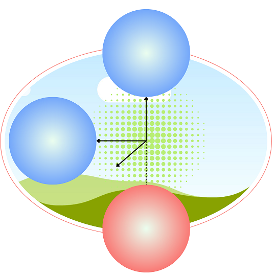From this we can derive three possible models of the internal structure of the electron (Fig. 1).

In the first model (Fig. 1a), two negative charges \(q\) rotate in two mutually perpendicular planes and, thus, hold each other by the magnetic fields generated during rotation. The second model (Fig. 1b) is quark and is suitable not only for the electron, but also for the proton [6]. Only one negative charge rotates in it, and the other two, opposite in sign, are located on the axis of this rotation, and are also held by the magnetic field of the first charge. The linear speed of the charge is equal to the speed of light, although due to a possible mass defect in reality it may be less. At the moment we are not considering the absolute distances between charges and their magnitude, although in the quark model they are known to some extent [6]. The next, third model, can have two or more charges, forming the tokamak principle (Fig. 1c).

Now let's check the result obtained based on this work. To do this, we will write out the basic formulas from there: \[ B_I^2 = B_1^2 + B_2^2 + 2 B_1 B_2 \cos(\alpha) \tag{1.11}\] \[ B_{II}^2 = 4 B_1 B_2 \sin(\alpha/2)^2 \tag{1.12}\] Here: \(B_1, B_2\) are the generators of the vector of the first magnetic field, \(\alpha\) is the angle between them. There is no singularity between these two vectors, so let's take their length to be onenovaya, which will lead us to the following calculations: \[ B_I^2 = 2 B_1^2\, (1 + \cos(\alpha)) \tag{1.13}\] \[ B_{II}^2 = 4 B_1^2 \sin(\alpha/2)^2 \tag{1.14}\] Considering that the angle \(\alpha\) is always equal to 90 degrees, let’s simplify these formulas even more: \[ B_I^2 = 4 B_1^2 \tag{1.15}\] \[ B_{II}^2 = 2 B_1^2 \tag{1.16}\] Let us also remind you that we are not considering absolute values ​​here, only relative ones. If we consider the square of induction, which is proportional to the field energy (formula 7), then an interesting picture emerges: the energy of MF₁ is twice as large as the energy of MF₂. The same result was obtained in [7, formula 17]. The solution to the so-called “4/3 problem” is also discussed there. based on such relationships. G. Nikolaev talks about solving this problem with the help of MF₂ energy in one of his interviews [8]. It also states that the energy of MF₁ should be twice the energy of MF₂.

The electron model presented here is not limited to solving some problems in electrodynamics, but also provides insight into some questions in quantum mechanics.

1. Quantized angular momentum of an electron
Such data were obtained by Stern and Gerlach as a result of an experiment with a magnet that deflected electrons either in one direction or the other at the same angle [9]. To do this, the electron itself must have a discrete magnetic moment, or a discrete value of magnetic induction. Let's look at formula (15). The square of the magnetic induction MF₁ is presented there. If you follow all the rules of mathematics, then the value of this induction to the first power will be as follows: \[ B_I = \pm 2 B_1 \tag{1.17}\] Pay attention to the sign in front of the right expression: it can be either a plus or a minus with equal probability. This means that in experiment [9], such systems will be equally deflected by a magnet in one direction or the other. By the way, to describe the shift of probability in one direction, you will need a more complex mathematical apparatus.

2. Electron spin
Let us turn our attention to formula (12), from which it follows that the period in it is obtained for two revolutions of the angle \(\alpha\). This means spin equal to ½ [10]. Here it is necessary to note that spin is formed exclusively due to MF₂ and without it this term has no meaning.

Physicists try to avoid this issue, although it would seem that everything here is obvious. The problem is that the electron has its own magnetic moment, which has been precisely proven by experiments [4]. This means that the charge in the electron must rotate, turning the electric field into a magnetic one, according to the principles of relativistic electrodynamics. But with such a point of view, all the foundations of electrostatics collapse. However, there is a fairly simple way out of this situation: the second MF, which is formed in the electron, is the source of the electric field [3, formula 10.9].

Our version is that the charge in the electron rotates, forming, as expected, a magnetic moment. At the same time, rotation forms an MF₂ around the electron, which in its induction properties is no different from an electric field. It is this that we, and our devices, perceive as an electric charge. In the second part we will talk about this in more detail.