

2025-01-14
Planetary electromagnetic waves
"If you want to understand the Universe, think in terms of Energy, Frequency, and Vibration." Nikola Tesla
 Our planet is not only unique in its nature and biosphere, but also has amazing wave properties. A whole ocean of waves of various natures and origins rages along the surface and inside the planet. These waves have a significant impact on all earthly processes, but despite this, they still remain poorly understood.
 In this paper, we will try to fill this gap and start with the Schumann resonance, a phenomenon that is currently known as low-frequency standing electromagnetic waves (SEW) propagating along the earth's surface [1]. The mechanism for the formation of such waves is very simple, since about 50 lightning bolts flash on our planet every second. These powerful discharges are the source of electromagnetic radiation that enters the natural resonator formed by the Earth's surface and the ionosphere(*). The length of this resonator is equal to the length of the planet's surface, so only waves that fit entirely within this length can remain in it. This is the property of the resonator!
If we convert the lengths of these waves into frequencies, it turns out that in our planetary resonator there can exist waves with the following frequencies: \[ f_n = {c \over \lambda} N \tag{1}\] where: \(c\) — the speed of light, \(\lambda\) — the circumference of our planet, \(N\) — the harmonic number: 1, 2, 3, …
For the first five harmonics, this formula gives the following series of frequencies: 7.5, 15, 22.5, 30, 37.5 Hz. But slightly different values were obtained experimentally: 7.83, 14.1, 20.3, 26.4, 32.4 Hz. The fundamental frequency, or the frequency of the first harmonic, — 7.83 Hz, differs from the calculated one because the calculation itself does not take into account the electrical and geographical properties of the earth, atmosphere and ionosphere, where the wave propagates, which gives a small error [1]. The formula given in the works of Schumann [1] is more consistent with the real series of frequencies, but has an unreal physical nature. In addition, it does not include a series of frequencies of the actually measured spectrum, which we will discuss further.
With the remaining harmonics, the values of which differ significantly from the calculated ones, things are even more interesting. And if we look at the full frequency spectrum in the range of 0-36 Hz (Fig. 1-2), we will additionally discover frequencies of approximately 1.6, 3, 4.8, 12, 25 Hz, as well as some others [2]. Their appearance in the spectrum cannot be explained from the point of view of the classical theory of a cavity resonator, even correcting it with additional electrical properties!
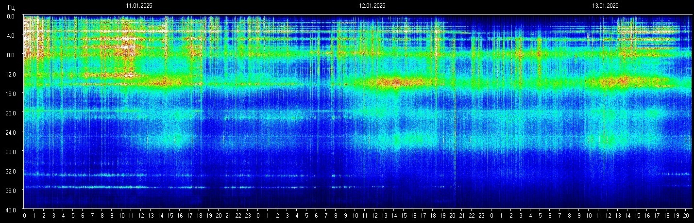 Fig. 1. Spectrum of planetary waves in the range of 0-40 Hz for three days | 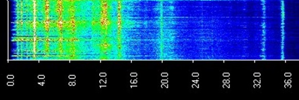 Fig. 2. A fragment of the spectrum, where additional frequencies are clearly visible |
Next, we will try to fill these gaps by putting forward only two assumptions. The first assumption is related to the presence of another source of such waves, and the second - to the mutual parametric capacitance between the ionosphere and the planet.
Two types of waves
In fact, when lightning strikes the earth, SEWs are formed not only along the surface of the planet, but also deep into it. For some reason, this second type of wave was forgotten, but it is they that provide the missing spectrum for the ultra-low frequency SEW (Fig. 1). Although Tesla wrote that it is possible to generate such standing waves with which the Earth enters into resonance, and which act as one of the terminals of a capacitor. He also claimed that the Earth can vibrate like a string [3]. Obviously, lightning discharges can also play the role of an exciting hammer.
 Fig. 3. Schematic representation of our planet consisting of a mantle and a core, and the conditional propagation of a wave inside it after a lightning strike. RE — radius of the planet |
Let's calculate at what frequencies our planet can vibrate, because here it plays the role of a resonator. To do this, you first need to calculate the speed of propagation of the wave, since inUnlike surface SEW, waves propagating inside the Earth will have a speed lower than the speed of light. This slowdown is due to the relative permittivity of the substance through which the electromagnetic wave propagates [4] \[v = {c \over \sqrt{\varepsilon \mu}} \tag{2}\] where: \(\varepsilon\) — relative permittivity, \(\mu\) — relative magnetic permeability, which for the mantle and core of our planet, on average, is close to unity. It follows that we need to focus primarily on the relative permittivity, which makes the formula for the SEW wave velocity in the ground quite simple: \[v = c / \sqrt{\varepsilon} \tag{3}\] This parameter has already been found in one of the earlier works [5, formulas 16-17], but there it is divided into two components: the permittivity of the planet's core \(\varepsilon_c\) and the permittivity of its mantle \(\varepsilon_m\). For further calculations, it is necessary to specify the permittivity of the core, since with strong heating of materials (and our core is heated to temperatures of about 6000 degrees), this parameter decreases. It will be determined precisely in further scientific research, but based on our hypothesis, it can be specified as follows: \(\varepsilon_c \approx 1.9\). We will leave the permittivity of the mantle the same \(\varepsilon_m = 6.5\). That is, part of the path the wave propagates at one speed, and part at another. From here it is easy to find the average speed of propagation of an electromagnetic wave inside the planet: \[v ={c \over 0.547 \sqrt{\varepsilon_c} + (1 - 0.547) \sqrt{\varepsilon_m} } \tag{4}\] Here:
0.547 is the relative distance from the center of the Earth to the boundary of its core (Fig. 3). Accordingly, 1-0.547 is the relative distance from the boundary of the core to the surface of the planet. Substituting the known values into (4), we finally obtain the speed of propagation of an electromagnetic wave in our planet: \[v \approx 0.52\, c \tag{5}\] That is, the average speed of propagation of an electromagnetic wave in the Earth is approximately half the speed of light. Now it is quite easy to find the resonant frequencies propagating inside the planet, by analogy with the frequencies propagating along it (formula 1): \[ F_n = {v \over 4\, R_E} N \tag{6}\] where: \(R_E\) — the radius of the Earth \(6.37\cdot 10^6\) m. And since the wave must first go in one direction, then reflect from the opposite edge and go back, we must multiply this radius by four. Let's substitute all known values into formula (6): \[ F_n \approx 6.2\, N \tag{7}\] From here follows a series of frequencies representing the SEW inside the Earth: 6.2, 12.4, 18.6, 24.8, … Hz. Probably, these are the electromagnetic vibrations of the Earth that Tesla spoke about.
Parametric planetary capacitor
It is possible that the upper layers of the atmosphere or outer space have an opposite charge and, together with the Earth, form a capacitor of enormous capacity. In this case, the oscillation period can be very small... N. Tesla's lecture from February 24, 1893.
 Fig. 4. Parametric planetary capacitor CW, formed between the surface of the planet and the ionosphere |
The surface wave propagates in a natural waveguide formed between the surface of the planet and the ionosphere, starting at a height of 60 km [6]. Compared to the Earth's diameter of 12,740 km, the waveguide height is only 0.2%, and it can also be considered as a capacitor, the plates of which represent the Earth and the ionosphere. In Figure 4, of course, such a capacitor is far from being drawn to scale. We will further call it a planetary capacitor \(C_W\).
Such a relatively thin planetary capacitor can be controlled (modulated) by an external electric field, which can be formed from the electric charge inside the planet \(q_E\). This field, in turn, is modulated by the SEW with a frequency from formulas (6-7). Thus, waves inside the planet, in fact, modulate waves in the planetary capacitor! The reverse process is also probable, the reality of which we will be able to learn about only after the start of studies of intraplanetary electromagnetic spectra.
By the way, the planetary capacitor is modulated by the same principle, but on the other hand - by the Sun. If the radiation flux from our star is large, then not only amplitude modulation occurs, but also frequency modulation (within small limits) [7]. This phenomenon is associated with the so-called magnetic storms, which have a significant impact on the well-being of people prone to weather sensitivity. We will talk about solar influence another time, but for now let's return to intraplanetary modulation.
Non-ideal spectrum
Knowing all of the above, we can obtain an approximate spectrum of the SEW in a planetary capacitor. To do this, first we will compose an equation that takes into account all of our previous developments: \[ S(t) = A(t) \cdot B(t) \\ A(t) = 1 + a_1 \sin(\omega_1 t) + a_2 \sin(2 \omega_1 t) + a_3 \sin(3 \omega_1 t) + \ldots \\ B(t) = 1 + b_1 \sin(\omega_2 t) + b_2 \sin(2 \omega_2 t) + b_3 \sin(3 \omega_2 t)+ \ldots \tag{8}\] Let's consider all the terms of this equation in detail. \(A(t)\) — these are surface SEWs in the planetary capacitor, propagating between the earth and the ionosphere, \(B(t)\) — these are intraplanetary SEWs. \(S(t)\) — these are electromagnetic waves in the planetary capacitor, in the fields of which you and I live. It is important here that they are obtained by mutual modulation of the amplitudes of surface and intraplanetary waves, which in the formula is achieved by simple multiplication of \(A(t)\) and \(B(t)\). The coefficients \(a_n, b_n\) reflect the relative amplitude of the corresponding harmonic; we have yet to find them. Also present in the formula are: \(\omega_1\) — angular frequency of the surface SEW, and \(\omega_2\) — angular frequency of the intraplanetary SEW.
To present this formula in the most general form, it would be necessary to add a phase under each sine, and to present the wave as an Euler function. But for a high-quality demonstration of the spectrum, this is not necessary.
We take only the first three harmonics for surface SEW, and the first four for intraplanetary SEW, and find the spectrum \(S(t)\) using MathCAD: 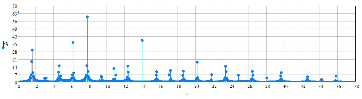 Fig. 5. Received spectrum of surface SEW in a planetary capacitor |
Figure 5 shows the calculated spectrum, where Gi is the amplitude of the i-th harmonic, i is the harmonic number, which corresponds, in this case, to the frequency in Hertz. The following data were used in the calculation: \(\omega_1 = 2\pi\cdot 7.8\), \(\omega_2 = 2\pi\cdot 6.2\). The coefficients were not specifically selected, and the following were chosen: a1 = 2, a2 = 0.4, a3 = 0.6, b1 = 1.2, b2 = 0.6, b3 = 0.4, b4 = 0.2. But even with them, it is clear that the spectrum began to more or less correspond to the real one, measured by the devices (Fig. 1-2 or here). Frequencies appeared in the spectrum, the absence of which puzzled us at the beginning of this note.
Additional spectrum lines
In Figure 2, in the range of 0..3 Hz, several weak spectrum lines can be seen. They can be associated with frequencies that we did not take into account in this work. For example:
- an intraplanetary wave can partially reflect from the core, both from its outer side and from the inner side;
- an intraplanetary wave can reflect several times from opposite sides.
Idealized spectrum
We can imagine a somewhat idealized spectrum consisting of the fundamental frequency of surface waves at 8 Hz, and intraplanetary waves with a fundamental frequency of 6 Hz and several of its harmonics: 12, 18, 24 Hz. Then the mutual modulation roughly fits into the spectrum actually obtained using the LNVA_20-24 device [8]. This spectrum is shown in Figure 6.
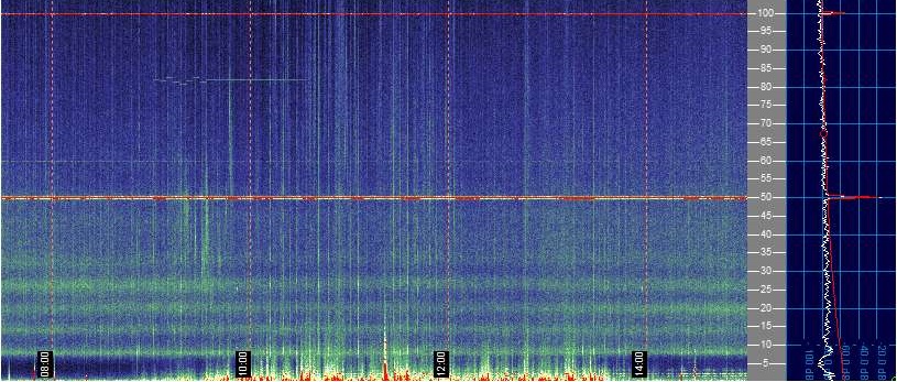 Fig. 6. Wave spectrum in a planetary capacitor obtained using the LNVA_20-24 device | 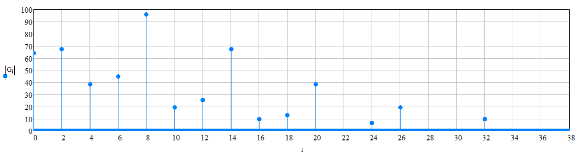 Fig. 7. Idealized spectrum of waves in a planetary capacitor obtained in MathCAD |
If we take the following data for MathCAD and formula (8): \(\omega_1 = 2\pi\cdot 8\), \(\omega_2 = 2\pi\cdot 6\), and the following coefficients: a1 = 3, b1 = 1.4, b2 = 0.8, b3 = 0.4, b4 = 0.2, then we will get the idealized spectrum in Figure 7. Of course, this spectrum is less accurate than the one shown in Figure 1, but it allows us to see the main patterns in it: the base frequency of the spectrum is approximately in the region 8 Hz, followed by harmonics, approximately proportional to \(8 + 6\cdot N\) Hz. The base frequency is formed by the surface planetary resonator, and the harmonics are formed by the intraplanetary resonator.
Connection with biorhythms
The frequency of the main Schumann resonance (7.83 Hz) is close to the frequency of alpha rhythms of the human brain, which are in the range of 7-14 Hz. Alpha rhythms are associated with relaxation, meditation, and increased concentration. It is believed that being in tune with the Schumann resonance can help improve cognitive function and reduce stress. Read more about these relationships in [9].
The Earth's natural electromagnetic vibrations can influence circadian rhythms — 24-hour biological cycles that govern sleep, wakefulness, and other physiological processes. Research suggests that Schumann resonances can synchronize with the body's internal rhythms.
Some scientists suggest that changes in the Schumann resonance caused by cosmic and geophysical factors may affect the ionic balance in the human body, affecting the nervous system and overall well-being.
There is evidence that strong changes in the electromagnetic activity of the Earth can correlate with changes in emotional state, heart rate and blood pressure in sensitive people. According to medical statistics, there is a clear correlation between magnetic storms and the success of operations.
All the data considered in this note indicate that the study of waves and frequencies of the planetary capacitor is in its infancy, but at the same time is a very important scientific direction both in the field of radio engineering and in the field of medicine.
(*)There is another, lesser-known source of such waves - the solar wind. It is a stream of charged particles continuously ejected from the upper layers of the Sun's atmosphere (the corona) into interplanetary space. About 95% of the solar wind consists of positively charged nuclei of hydrogen atoms.
Materials used
- Wikipedia. Schumann resonances.
- Space Observing System. [Web Archive]
- N. Tesla. On Electricity. Electrical Review, January 27, 1897.
- Professor V. V. Mayer. Electromagnetic Waves. 4.4. Velocity of an Electromagnetic Wave in a Vacuum.
- Gorchilin V. Solitary Capacity of the Planet Earth.
- Wikipedia. Ionosphere.
- Space Observing System. [Web Archive]
- Marconi Antenna + Geophone. [Web Archive]
- About interaction of Schumann waves with the human brain. [Web Archive]