

2023-08-18
Energy spectrum of a moving point
Mathematics is our connection to reality!
This material is intended for people seeking and wishing to plunge into the world of the unknown.
If you go headlong into it, then it can turn your mind and many ideas about our reality.
Quantum mechanics has come closest to the world of chances and probabilities, but even it does not answer many questions about the causes of particle behavior.
For example, why, when accelerating a group of fermions (protons, neutrons, electrons, etc.), their energy spectrum is strongly distributed over energy levels,
although the force applied to each of them is the same?
Yes, you can refer to the uncertainty principle [1] and the wave function [2], but this does not change the main question - why.
The same question can be asked about the experiment with two slits [3], to which we can add one more: how does the operator influence this experiment?
This may seem strange, but mathematics can give an answer to it if it applies its powerful statistical apparatus, some of which we will use in this work.
Also, here we will express several hypotheses about the particle and antiparticle, their energy spectrum in motion, and a new look at the energy balance.
In this note, we will consider a hypothetical particle as a mathematical point based on the hypothesis of single space,
in which there are many dimensions, where all the main transformations take place.
In terms of quantum mechanics, such a particle has zero spin.
According to our hypothesis, it is in multidimensional space that all possible accidents and probabilities arise, which, when projected onto our three-dimensional spatial world, sometimes form it in the most bizarre way.
Warm-up for the mind
Do you think that mathematics does not correspond to our reality?
Then read this note, where the influence of the operator on the probability of a plus or minus falling out completely changes the picture of the experiment.
This is not enough? Then think and say what is the sum of a series of natural numbers, where their number tends to infinity.
That is, how much
\[ 1 + 2 + 3 + 4 + 5 +\ldots =\, ? \]
Of course, infinity, you say. And you will be wrong :)
The correct answer is [4]:
\[ 1 + 2 + 3 + 4 + 5 +\ldots = \boldsymbol{ -\frac{1}{12} } \]
If you haven't bought this idea yet, then at least
it's time to think about the fact that our idea of reality and our reality are completely different things!
And we're not talking about reality yet :)
Point movement
Now, after a small digression and a warm-up for the mind, let's return to the point that moves in our space with the speed \(v\).
According to the unit space hypothesis, the global velocity vector (GVV) applies to such a point:
\[\mathbf{V} = \frac{\mathbf{v}}{\gamma} \tag{1}\]
Here: \(\mathbf{v}\) -- multidimensional velocity vector (non-normalized GVV)
\[\mathbf{v} = c \left\{\pm 1,\, \pm \beta,\, \pm \beta^2,\, \ldots ,\, \pm \beta^n \right\} \tag{2}\]
where \(c\) is the speed of light, \(\gamma\) - Lorentz factor
\[\gamma = 1 / \sqrt{1 - \beta^2}, \quad \beta = v/c \tag{3}\]
acting in formula (1) as a function normalizer.
Using the theorem about transforming a scalar into a vector, we expanded the Lorentz factor into a multidimensional space and normalized it.
Further, we assume that all actions with a point take place in such a space, and our three-dimensional - is formed from it by reflection (projection or convolution).
If our point (or particle) has a mass, then during its movement it acquires momentum, but not classical, but
global momentum vector (GPV) built on the same principles:
\[\mathbf{P} = m_0 \mathbf{v} \tag{4}\]
In our works, the number of members of the series is taken, starting from zero.
The time coordinate is responsible for the zero term, and the speed in our real space is usually responsible for the first term.
Signs in front of all members of the series, except for the first one, are unknown to us and, in the general case, may be random.
Then, taking into account the unidirectional movement of time and the known direction of the first coordinate (velocity in real space), this vector will be written as follows:
\[\mathbf{v} = c \left\{1,\, \beta,\, \pm \beta^2,\, \ldots,\, \pm \beta^n \right\} \tag{5}\]
Obtaining the energy of a point consisting of GVV and GPV comes down to multiplying these quantities:
\[ \hat E = \mathbf{P} \mathbf{V} = {m_0 c^2 \over \gamma} \left(1 + \beta^2 + \sum \limits_{n=2}^N \pm \beta^{2n} \right) \tag{6}\]
Note that before each term of the sum in (6), plus or minus values can appear with a known probability of such an event.
And in the most general form, plus or minus can appear before the zero member of the series, before the unit in (6), because the direction of the time axis is also generally unknown to us.
But more on that later.
Previously, we have already considered the energy obtained from the global momentum and global velocity,
and it exactly equaled Einstein's mass-energy (formula 1.10).
But when deriving them, it was assumed that the terms for the corresponding speeds \(\mathbf{v}\) are the same, and therefore such a simplified approach to the problem was considered.
Here we consider a more generalized version of this approach,
for which we will use the ready-made mathematical model of random sign-alternating series (SZPR) from of this work.
Based on this, we rewrite the function (6) by adding the experience number \(k\)
\[ \hat E_k = {m_0 c^2 \over \gamma} \left(1 + \beta^2 + \sum \limits_{n=2}^N \pm \beta^{2n} \right) \tag{7}\]
and normalize it for better perception:
\[ E_k = \sqrt{1 - \beta^2} \left(1 + \beta^2 + \sum \limits_{n=2}^N \pm \beta^{ 2n} \right), \quad E_k = {\hat E_k \over m_0 c^2} \tag{8}\]
Further, we will speak only about the normalized energy.
That is, each experience contains the sum of a row with random signs, so its sum is different every time.
We write the results of the experiments in two arrays, with positive and negative sums (details).
Based on this, we construct the energy spectrum of the function obtained above, where the probability of occurrence \(\pm\) is equal to ½:
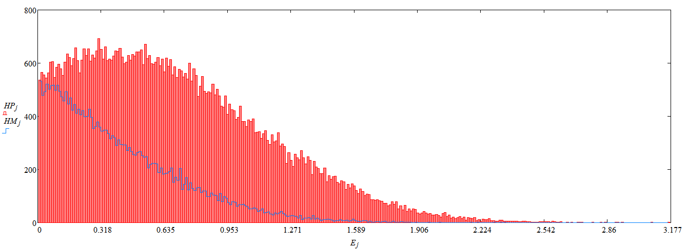
Fig.1. Energy spectrum of function (8) at β=0.98. Red graph -- positive results, blue graph -- negative results
|
In this figure, HP and HM are data from the plus and minus array, respectively, summed over a certain energy range Ej,
where j is the range number.
For example, in the energy range of 0.318, there were about 650 positive results from experiments according to formula (8), and about 350 negative results, with a total number of experiments \(K=100000\).
The more experiments we carry out, the more the maximum energy will approach the value of the Lorentz factor, that is, to \(1 / \sqrt{1 - \beta^2}\).
Energy balance
Let's look at the total sum of energies from the HP and HM arrays obtained above, and derive the average energy from this:
\[ S = {1 \over K} \sum (HP_j + HM_j) \tag{9}\]
For the above formula, where the probability of \(\pm\) appearing before the terms of the series is ½, and the resulting graph (Fig. 1),
this amount will be: \(S=0.39\).
Apparently, in real space (in our nature) there should be a balance of energies, which, in this case, determines the sum according to formula (9) equal to one.
In other words, no matter how we move a point in space, its average normalized energy will always be equal to one:
\[ S = 1 \tag{10}\]
Further, we will call the spectrum unity if its average normalized energy is equal to unity: \(S=1\).
We introduce this postulate as a consequence of the energy of the global velocity vector.
But if for GVV this property is derived directly from its formula (its square),
then to obtain a unit normalized energy, it is necessary, to a certain extent, to influence the probability of \(\pm\) appearing before the terms of the series.
For example, with β=0.98, you need to slightly increase the probability of pluses appearing over minuses:
\[ E_k = \sqrt{1 - \beta^2} \left(1 + \beta^2 + \sum \limits_{n=2}^N sign(rand(1) - 0.435)\, \beta^{2n} \right), \quad S = 1 \tag{11}\]
Where: \(sign(rand(1) - 0.435)\) is the function of the appearance of a plus or minus with a shift towards plus.
The graph of the resulting function with a biased probability will be as follows:
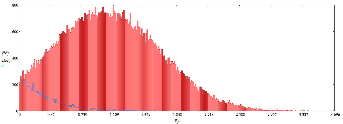
Fig.2. Unit spectrum of function (11) at β=0.98 and balanced energy S=1
|
In fact, we have the spectrum from Figure 1, but with a shift to the positive region (more).
Single Spectrum
The spectrum is unit if if its average normalized energy is equal to unity.
This property directly follows from the energy conservation law [5].
Such a spectrum is quite understandable, when there are many particles (points), then each of them can have its own energy, which in total gives such a distribution (Fig. 2).
But what about one particle?
The explanation here can be the only possible one: any particle that has been given an impulse carries all possible energy options according to (11),
what can be called reality for her.
In reality, as we know, there are many possibilities, sometimes even completely opposite in sign.
The manifestation of a specific measurable energy occurs when a particle passes from reality to our reality,
which happens, for example, in the slit experiment [2] or in other measurements.
The transition of reality into reality occurs when reflection of multidimensional space onto our three-dimensional one.
In our opinion, in order to maintain the balance of energy, or to preserve a single spectrum, nature is forced, in some cases, to give birth to antiparticles.
Moreover, such a particle is apparently born not at any negative energy (see Fig. 2, blue graph), but only in the case of the opposite direction of the time axis (zero coordinate).
Therefore, there are much fewer antiparticles.
This, of course, contradicts some provisions of the Big Bang theory, for example, in terms of the annihilation of matter.
In our hypothesis, the reason for the birth of an antiparticle is the law of conservation of energy!
Negative energy
Formula (11) assumes the appearance of some experiments with negative energy values.
In physics, such energy is considered in two aspects.
The first model was proposed by Niels Bohr to explain the motion of an electron around its orbit.
According to this model, the energy of an electron in orbit is negative, which prevents it from leaving it [6].
The second interpretation of negative energy follows from quantum mechanics, where such energy belongs to the antiparticle [7].
Both explanations are suitable for our hypothesis.
Let us explain with an example in which some assumptions are made to qualitatively show the connection between our hypothesis and reality.
Let's assume that we accelerate our particles, which have a charge, using a high-voltage accelerator [8, fig. 1.2.1],
reaching sufficiently high energies at which β is close to unity.
Despite the fact that electrons are not quite suitable for analogy with our particles, their spectrum after acceleration [8, fig. 2.4.2] resembles graph 2.
More accurate spectra can be obtained by taking into account the internal energy of the electron, and increasing their number in the experiment by orders of magnitude.

Fig.3. Acceleration of electrons in an electric field U-...U+. Some electrons collide with exotic particles and change direction (\(v_4 \to v_4^{'}\))
|
In addition, accelerated particles always have a spread in the directions of motion [9, fig. 2.5], and in order to explain this, negative energy is needed.
A small part of the particles that have negative energy (Fig. 2, blue graph) form the so-called "exotic particles" [10],
for example, positronium, consisting of an electron and a positron [11], with a lifetime of about 0.12 ns.
Since their energy is in a bound state, they are stationary relative to moving particles with positive energy.
When the first and second types of particles collide, the moving particles deviate from the acceleration axis (Fig. 3).
How the point moves
Let's analyze: if in function (8) almost everything is random, then what changes when we start moving a point in space?
We have already talk that such a displacement can always be represented as two coordinates:
one spatial and one temporal, that is, the movement of a point in space at any moment of time is one-dimensional.
This fact is missed by modern science, but in vain.
Let's call this coordinate direction.
In our case, one spatial coordinate is represented by the first term of the sum (5) in the form \(\beta\) with a plus sign.
All other axes, in general, can have a random direction and random sign values.
It turns out that when moving a point in space, we only affect the probability of the sign in front of the directing coordinate.
And if the conditions of the unit sum (11) are also imposed on formula (8), then we, depending on the speed, albeit to a small extent, we also influence the probability of the sign in front of the other coordinates.
But for a particle there is no difference how exactly the probability changes, by the application of external energy or, for example, by the power of the operator's thought.
This idea should be devoted to a separate work, but for now let's note that the movement of objects in space by means of telekinesis, apparently, is not such a fantasy.
And, mind you, this follows not from physics, but from mathematics!
It is worth recalling that if the influence on the sign probability is large, then we will get a unit degenerate spectrum,
which is obtained when the experimenter influences the quantum experiment (more).
In this case, science says that the particle begins to show corpuscular properties, although before that it showed quite wave properties.
Relationship between the wave function and the global velocity vector
Modern physics knows the physical meaning of only the square of the wave function [12].
Let's try to connect the wave function \(\Psi\) and the global velocity vector
by multiplying two GVV vectors, provided that the plus-minus sets in each of the factors are different,
and to achieve the condition of property (10), one can influence the probability of their occurrence (shift its spectrum):
\[ F_k = \frac{1}{c^2} \mathbf{V} \cdot \mathbf{V}^{*} = \frac{1}{\gamma^2 c^ 2} \sum \limits_{n=0}^{\infty} \pm \mathbf{j_n} \beta^n \cdot \sum \limits_{n=0}^{\infty} \pm \mathbf{j_n} \beta^n \tag{12}\]
If one or several directions are precisely known, for example, as in formula (5), then these terms of the series receive not a random, but a constant sign.
Example:
\[ F_k = \frac{1}{c^2} \mathbf{V} \cdot \mathbf{V}^{*} =
\frac{1}{\gamma^2 c^2} \left(\mathbf{j_0} + \mathbf{j_1} \beta^2 + \sum \limits_{n=2} ^{\infty} \pm \mathbf{j_n} \beta^n \right)
\cdot \left(\mathbf{j_0} + \mathbf{j_1} \beta^2 + \sum \limits_{n=2}^{\infty} \pm \mathbf{ j_n} \beta^n \right) \tag{13}\]
Using property (10), we can derive the sum of all experiments whose number is equal to \(K\)
\[ S = {1 \over K} \sum \limits_{k=0}^K F_k = \frac{1}{c^2 K} \sum \limits_{k=0} ^K \mathbf{V} \cdot \mathbf{V}^{*} = \int \limits_{\vee} \Psi \cdot \Psi^{*}\, d \vee = 1 \tag{14}\]
which is also equal to the probability of detecting a particle in the entire space with a volume \(\vee\) [12].
To achieve accurate results, \(K\) must go to infinity.
An obvious connection between \(\Psi\) and GVV is shown in expression (14),
whence one can try to find the physical meaning of the wave function in the first degree.
Slow down
Earlier in this note, we worked with velocities close to the speed of light.
But let's see how the energy spectrum changes at lower speeds.
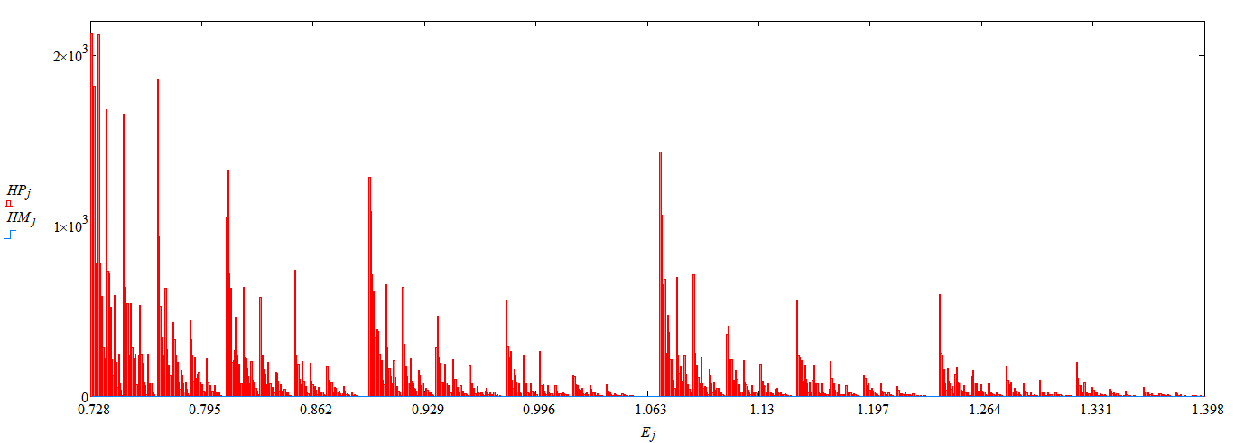

Fig.4. Unit spectrum of function (11) at β=0.7, S=1.
Bottom - array data EPk with positive test results, where each point is one test |
Approximately from β=0.8 and up to β=0.5, a discrete spectrum begins to appear (Fig. 4), which degenerates into a four-band
(two bands - positive spectrum, two bands - negative spectrum) at a lower velocity value (Fig. 5).
In fact, if we consider one of its bands, we will find that it also consists of several discrete bands, and so on. to infinity,
but because β is small, they are close to each other.
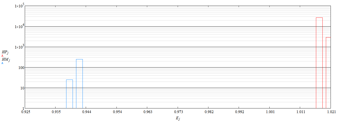
Fig.5. Unit spectrum of function (11) at β=0.2, S=1
|
At low speeds, in order to comply with principle (10), it is necessary to mix points with negative values of the time axis, which, in theory, should correspond to antiparticles.
For example, for β=0.2, formula (11) might look like this:
\[ E_k = \sqrt{1 - \beta^2} \left(sign(rand(1) - 0.0085)\, + \beta^2 + \sum \limits_{n=2 }^N sign(rand(1) - 0.9)\, \beta^{2n} \right) \tag{15}\]
Here \(sign(rand(1) - 0.0085)\) is, in fact, responsible for the birth of antiparticles in a ratio of about 1/60.
For very low speeds, to which we are accustomed in our world, the spectrum turns into almost single-band,
Athe number of antiparticles that must restore the energy balance is reduced by β2 times.
Conclusions
In this work, it was possible to connect the theoretical hypothesis about single space with real data concerning the spectra of moving particles.
Small differences are explained by the presence of internal energy, and hence the internal motion of real particles, about which little is known to physics yet.
The manifested spectrum is the result of the balance of energies in nature, and the hypothesis of the presence of multiple dimensions is quite suitable for its explanation.
It is in them that all processes take place, which, reflecting on our three-dimensional spatial world, give inexplicable, at first glance, results.
The probabilistic nature of the movement of a point in space is also provided by the reflection of the real world on our real one.
At the same time, for the movement itself, it doesn’t matter how exactly the probability changes: by an external force effect or by another way the operator influences it.
The note gives some ideas about the reason for the appearance of antiparticles, as a way of nature to comply with the law of conservation of energy.
Antiparticles, together with particles, can form exotic atoms, which, being in the path of particles, can deflect them in different directions.
This, for example, completely explains the angular distribution of the bremsstrahlung of an electron beam.
Despite the results achieved, the presented hypothesis requires further elaboration both in terms of mathematics and in terms of its alignment with known processes in our reality.
Materials used
- Wikipedia. Principle uncertainty.
- Wikipedia. Double-slit experience.
- Wikipedia. Wave function.
- Wikipedia. natural numbers.
- Wikipedia. Law conservation of energy.
- Wikipedia. Borovskaya atom model.
- Wikipedia. field theory.
- A. P. Chernyaev, M.A. Belikhin, M. V. Zheltonozhskaya. Introduction to the physics of charged particle accelerators. [PDF]
- Ji Dollar. Beams of particles. Chapter 2. [Site]
- Wikipedia. Exotic atom.
- Wikipedia. Positronium.
- Wikipedia. Wave function.