

2026-08-01
Geometric origin of electric force
Wave electricity is based on the assumption that the observed properties of particles and the laws of their motion must derive from a single geometric structure. In this concept, mass, energy, external motion, and internal state are viewed not as independent quantities, but as different projections of a single, unified geometric structure. The model's fundamental principles and existing results are summarized in the review paper "Introduction to Wave Electricity."
But if geometry truly underlies physical reality, it should derive not only the properties of individual particles but also the laws of interaction between particles. One of the most important tests of this idea is Coulomb's law. Therefore, the goal of this article is to first derive from geometry the very principle of interaction, the dependence of energy on distance, and the inverse-square law—and only then demonstrate under what conditions this general result takes the form of Coulomb's law.
The geometric principle of attraction: two projections of the same internal energy.
In previous work, the internal frequency of a particle was related to its observed rest energy. Now let's consider the next step: can the same internal energy create a dependence on the distance between two objects—even before introducing charge, permittivity, and Coulomb's law?
The basic idea is that an external object does not see the entire internal geometry of the particle at once. Two close internal branches are observed at slightly different angles. Their projections almost cancel out, but a small difference remains between them. It is this difference that creates the distance-dependent part of the energy.
\[ \tag{1} \boxed{ \text{two close branches} \;\longrightarrow\; \text{difference in projections} \;\longrightarrow\; \text{interaction energy} \;\longrightarrow\; \text{force} } \] First, we derive the general principle of attraction without charges. Only then can we compare the resulting coefficient with the known electrostatic coefficient.
1. Two Close Internal Branches
The premise of this construction was previously discussed in the work on two levels of closed electron motion and the parameters of the Bohr atom. There, the single state of the electron is represented as a combination of internal and external mutually orthogonal rotations, and the observed parameters arise as projections of this composite motion. Here, we develop the same idea in spatial form: we consider not two independent electrons, but two close branches of a single internal state and investigate the small difference in their projections onto an external object.
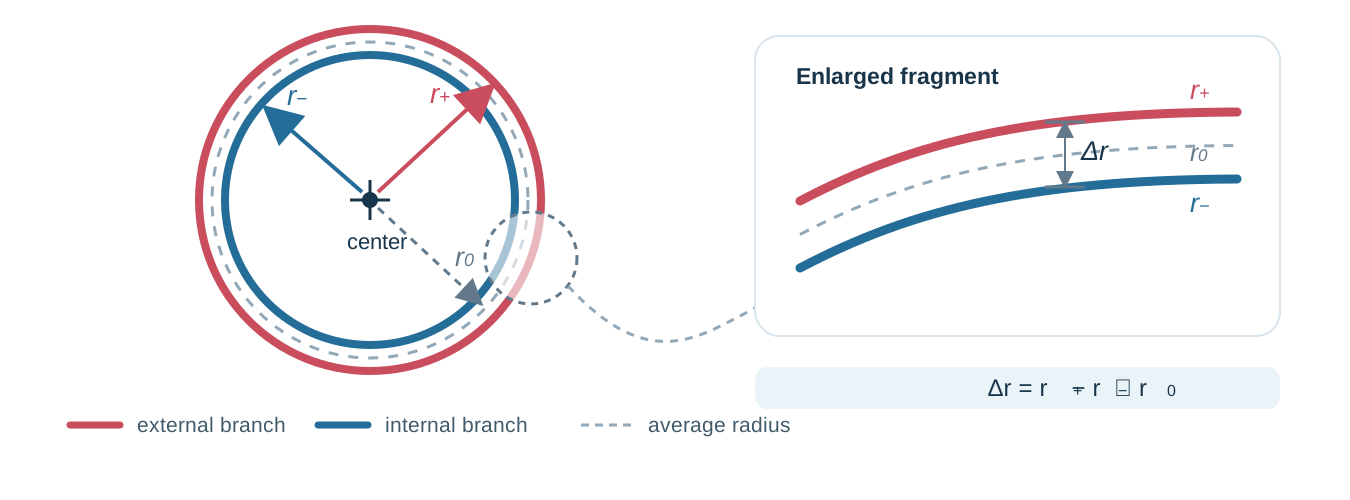
Let the internal state of an object contain two close spatial branches with characteristic radii \(r_+\) and \(r_-\). It is convenient to imagine them symmetrically with respect to the average radius \(r_0\):
\[ \tag{2} \begin{aligned} r_+&=r_0+\frac{\Delta r}{2}, \\ r_-&=r_0-\frac{\Delta r}{2}. \end{aligned} \] The distance between the branches is
\[ \tag{3} \Delta r=r_+-r_-, \qquad \Delta r\ll r_0. \] Here, we are not talking about two positions of the external particle, but about two components of a single internal state. In more general geometry, \(\Delta r\) should be understood as the effective separation of the branches in the projection direction. Therefore, the branches may have not only different radii: they may be slightly offset, tilted, or located in different internal planes.
2. One external object — two projection angles
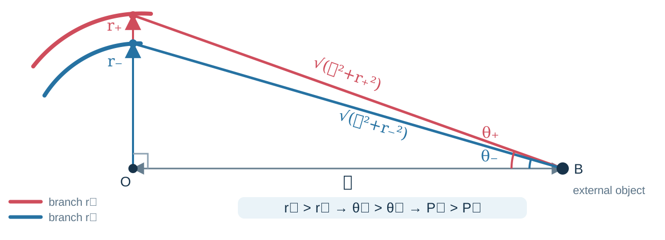
Let's place the second object at a distance \(\ell\) from the center of the first. For the two internal branches, two slightly different angles arise: \(\theta_+\) and \(\theta_-\). Their geometric projection coefficients are equal
\[ \tag{4} P_+(\ell) = \sin\theta_+ = \frac{r_+}{\sqrt{\ell^2+r_+^2}}, \] \[ \tag{5} P_-(\ell) = \sin\theta_- = \frac{r_-}{\sqrt{\ell^2+r_-^2}}. \] Each projection individually is large compared to their difference. For external interaction, the uncompensated remainder is significant:
\[ \tag{6} \boxed{ \Delta P(\ell) = P_+(\ell)-P_-(\ell) } \] \[ \tag{7} \Delta P(\ell) = \frac{r_+}{\sqrt{\ell^2+r_+^2}} - \frac{r_-}{\sqrt{\ell^2+r_-^2}}. \] Formula (7) is derived only from geometry. It does not yet include energy, force, or charge. The external object also does not "receive" the internal radius of the particle: it only distinguishes two internal branches at slightly different values.angles.
3. What exactly can be projected in energy?
Energy as a number is a scalar, so it is impossible to literally project the scalar itself. In the model, a directed internal energy state is projected, and energy is its modulus.
Let the internal frequency correspond to the full energy scale.
\[ \tag{8} E_0=h\nu_{\mathrm{int}} = \hbar\omega_{\mathrm{int}}, \qquad \omega_{\mathrm{int}}=2\pi\nu_{\mathrm{int}}. \] If \(\widehat{\mathbf u}_\pm\) are the directions of two internal branches, then the directed energy states can be written as
\[ \tag{9} \boldsymbol{\mathcal E}_\pm = E_*\widehat{\mathbf u}_\pm, \] where \(E_*\) is the energy scale already accessible to external space. Its origin will be clarified in the next section.
Let \(\widehat{\mathbf n}_{\pm}(\ell)\) define the directions from the external object to the corresponding internal branches. These directions are slightly different, so the same internal energy state receives two close transverse projection coefficients.
\[ \tag{10} E_+^{\mathrm{proj}} = \boldsymbol{\mathcal E}_+ \cdot \widehat{\mathbf n}_+(\ell) = E_*\sin\theta_+ = E_*P_+(\ell). \] \[ \tag{11} E_-^{\mathrm{proj}} = \boldsymbol{\mathcal E}_- \cdot \widehat{\mathbf n}_-(\ell) = E_*\sin\theta_- = E_*P_-(\ell). \] These are not two independent total energies \(E_*\). They are two geometric components of a single internal energy scale. Therefore, their difference manifests itself externally:
\[ \tag{12} \boxed{ \Delta E_{\mathrm{proj}}(\ell) = E_*\Delta P(\ell) } \] \[ \tag{13} \Delta E_{\mathrm{proj}}(\ell) = E_* \left[ \frac{r_+}{\sqrt{\ell^2+r_+^2}} - \frac{r_-}{\sqrt{\ell^2+r_-^2}} \right]. \] Thus, the transition from geometry to energy does not require introducing an arbitrary dimensional constant: the dimensionless coefficient \(\Delta P\) projects the already existing internal energy scale.
The relationship between the directed state and energy, expressed by formulas (9)–(12), is the physical principle of the model. Geometry unambiguously yields \(\Delta P(\ell)\), but trigonometry alone does not prove that this projection should be observed as the interaction energy.
4. Two Consecutive Projections
In the article on mass, the internal energy \(E_0\) was no longer directly identified with the rest energy. First, it undergoes a transverse Doppler projection with a coefficient \(\alpha_{\mathrm{fs}}\):
\[ \tag{14} E_* = \alpha_{\mathrm{fs}}E_0 = \alpha_{\mathrm{fs}}\hbar\omega_{\mathrm{int}} = m_ec^2. \] It is the observed energy \(E_*=m_ec^2\), and not the original energy \(E_0\), that then participates in the external spatial projection. The resulting sequence is:
\[ \tag{15} \boxed{ \begin{gathered} E_0=\hbar\omega_{\mathrm{int}} \\ \downarrow\quad \alpha_{\mathrm{fs}} \\ E_*=m_ec^2 \\ \downarrow\quad \Delta P(\ell) \\ \Delta E_{\mathrm{proj}}(\ell) = m_ec^2\Delta P(\ell). \end{gathered} } \] The first projection converts the intrinsic frequency into the observed resting energy. The second selects that small portion of this energy that depends on the relative positions of the two objects.
The origin of the first transition is discussed in detail in the article "Mass as a Transverse Doppler Projection of Internal Frequency".
5. Potential Energy of a Consistent State
The difference in energy projections \(\Delta E_{\mathrm{proj}}\) is a positive value. To obtain an attractive state, it is necessary to determine how this value enters into the balance of internal and external energies.
We will call a mutual state of two objects consistent if an increase in projection agreement decreases the potential energy of the system. Then
\[ \tag{16} \boxed{ U_{\mathrm{att}}(\ell) = -\Delta E_{\mathrm{proj}}(\ell) = -E_*\Delta P(\ell) } \] The minus sign here is not yet a charge sign. It denotes only the selected branch of mutual coordination: when the potential energy decreases, the released part of the internal energy can be converted into external motion.
The exact potential energy of such a state is
\[ \tag{17} U_{\mathrm{att}}(\ell) = -E_* \left[ \frac{r_+}{\sqrt{\ell^2+r_+^2}} - \frac{r_-}{\sqrt{\ell^2+r_-^2}} \right]. \] Formula (16) is the second physical principle of this construction. In the future, it is desirable to obtain its sign directly from the structure of \(J\), the mutual orientationation of idempotent branches or the minimum measure of misalignment of global vectors. In this derivation, we first explore all the consequences of this principle.
6. Far Field and the Law of \(1/\ell\)
If the distance between objects significantly exceeds the inner radii,
\[ \tag{18} \ell\gg r_+,r_-, \] then the projection coefficients take a simple form:
\[ \tag{19} P_\pm(\ell) \approx \frac{r_\pm}{\ell}. \] Their difference is
\[ \tag{20} \Delta P(\ell) \approx \frac{r_+-r_-}{\ell} = \frac{\Delta r}{\ell}. \] Therefore, the potential energy of the consistent state becomes
\[ \tag{21} \boxed{ U_{\mathrm{att}}(\ell) \approx -E_*\frac{\Delta r}{\ell} } \] The dependence \(1/\ell\) is not introduced here as a predetermined potential. It arises from the difference in the angular projections of two close internal branches. The quantities \(\Delta r\) and \(\ell\) play different roles: the internal separation determines the interaction amplitude, while the external distance determines its spatial weakening.
7. From Energy Redistribution to Force
We use the model's basic postulate of the constancy of the total energy:
\[ \tag{22} E_{\mathrm{ext}} + E_{\mathrm{int}} = \operatorname{const}. \] The distance-dependent part of the internal energy is represented by the quantity \(U_{\mathrm{att}}(\ell)\). Therefore,
\[ \tag{23} dE_{\mathrm{ext}} = -dU_{\mathrm{att}}. \] Let's choose the direction in which the distance \(\ell\) increases as positive. The work done by the radial force is equal to
\[ \tag{24} dE_{\mathrm{ext}} = F_\ell\,d\ell. \] Therefore,
\[ \tag{25} \boxed{ F_\ell = -\frac{dU_{\mathrm{att}}}{d\ell} } \] For the far region, we substitute formula (21):
\[ \tag{26} \boxed{ F_\ell \approx -E_*\frac{\Delta r}{\ell^2} } \] Since \(E_*>0\), \(\Delta r>0\), and \(\ell>0\), we obtain \(F_\ell<0\). Given the chosen direction, this means a decrease in the distance between objects, i.e., attraction.
Thus, the general inverse-square law is obtained without introducing charge:
\[ \tag{27} \boxed{ |F_\ell| \approx E_*\frac{\Delta r}{\ell^2} } \] 8. Two Different Gradients
In this mechanism, it is important not to confuse the internal finite difference and the external spatial gradient. The internal quantity
\[ \tag{28} G_{\mathrm{int}}(\ell) = \frac{E_+^{\mathrm{proj}}-E_-^{\mathrm{proj}}} {r_+-r_-} = \frac{\Delta E_{\mathrm{proj}}}{\Delta r} \] characterizes the difference between two close branches. It defines the amplitude of the uncompensated energy projection. The external force is determined by another operation:
\[ \tag{29} F_\ell = -\frac{dU_{\mathrm{att}}}{d\ell}. \] Therefore, the two internal branches are not two external points between which a force directly acts. They create a difference in energy projections dependent on \(\ell\), and the external gradient of this energy creates movement.
\[ \tag{30} \boxed{ \Delta r \;\longrightarrow\; \Delta P(\ell) \;\longrightarrow\; \Delta E_{\mathrm{proj}}(\ell) \;\longrightarrow\; U_{\mathrm{att}}(\ell) \;\longrightarrow\; F_\ell } \] 9. Exact Formula and Far-Range Boundary
If we do not use the approximation \(\ell\gg r_\pm\), differentiating formula (17) yields
\[ \tag{31} F_\ell = -E_*\ell \left[ \frac{r_+}{\left(\ell^2+r_+^2\right)^{3/2}} - \frac{r_-}{\left(\ell^2+r_-^2\right)^{3/2}} \right]. \] At large distances, the expression in square brackets is positive, and formula (31) transforms into the law of attraction (26). However, in the immediate vicinity of the inner radii, the behavior of the exact formula is more complex.
For two very close branches, the difference can be expanded in terms of a small parameter \(\Delta r\):
\[ \tag{32} \Delta P(\ell) \approx \frac{\partial}{\partial r} \left( \frac{r}{\sqrt{\ell^2+r^2}} \right)_{r=r_0} \Delta r = \frac{\ell^2\Delta r} {\left(\ell^2+r_0^2\right)^{3/2}}. \] Then the energy and force take the form
\[ \tag{33} U_{\mathrm{att}}(\ell) \approx -E_* \frac{\ell^2\Delta r} {\left(\ell^2+r_0^2\right)^{3/2}}, \] \[ \tag{34} F_\ell \approx -E_*\Delta r\, \frac{\ell\left(\ell^2-2r_0^2\right)} {\left(\ell^2+r_0^2\right)^{5/2}}. \] From formula (34), it is clear that simple two-branch geometry predicts zero force near
\[ \tag{35} \ell_0\approx\sqrt{2}\,r_0. \] For \(\ell>\ell_0\), the force has the sign of attraction, and for \(\ell<\ell_0\), this simple formula changes sign. This cannot be considered an established physical effect.ktom. Two interpretations are possible: either the model predicts a short-range repulsive region, or spatial projection (7) is only applicable in the far region and must be supplemented with full geometry \(J\) at short distances. Only the reliable region \(\ell\gg r_0\) is used to derive the inverse square law.
10. How close are the internal branches?
For an electron, the natural mean internal scale is the reduced Compton length.
\[ \tag{36} r_0 = \bar\lambda_C = \frac{\hbar}{m_ec} = \frac{r_e}{\alpha_{\mathrm{fs}}}. \] If the effective separation of the branches is equal to the classical radius of the electron,
\[ \tag{37} \Delta r=r_e, \] then their relative distance is small:
\[ \tag{38} \boxed{ \frac{\Delta r}{r_0} = \alpha_{\mathrm{fs}} \approx 0.007297 } \] In other words, the distance between the branches is approximately \(0.73\%\) of their average radius, and each branch deviates from the average value by approximately \(0.365\%\). Therefore, the condition \(\Delta r=r_e\) does not contradict the assumption of two almost coinciding internal trajectories.
\[ \tag{39} \begin{aligned} r_0&\approx3.86159\cdot10^{-13}\ {\rm m}, \\ r_+&\approx3.87568\cdot10^{-13}\ {\rm m}, \\ r_-&\approx3.84750\cdot10^{-13}\ {\rm m}. \end{aligned} \] It is important to use the standard notation here: \(r_e/\alpha_{\mathrm{fs}}\) is the reduced Compton length of the electron. The Bohr radius has a different scale:
\[ \tag{40} a_0 = \frac{r_e}{\alpha_{\mathrm{fs}}^2}. \] The relationship between these radii is discussed in detail in the article "Parameters of the Bohr Atomic Model".
11. Numerical normalization without introducing charge
In the far field, the coefficient of the general law of attraction is
\[ \tag{41} K_{\mathrm{geom}} = E_*\Delta r. \] For an electron, \(E_*=m_ec^2\). If the geometry of the internal branches yields \(\Delta r=r_e\), then
\[ \tag{42} K_{\mathrm{geom}} = m_ec^2r_e. \] Using a known ratio
\[ \tag{43} r_e = \alpha_{\mathrm{fs}} \frac{\hbar}{m_ec}, \] get
\[ \tag{44} \boxed{ K_{\mathrm{geom}} = m_ec^2r_e = \alpha_{\mathrm{fs}}\hbar c } \] \[ \tag{45} K_{\mathrm{geom}} \approx 2.30708\cdot10^{-28}\ {\rm J\,m}. \] Up to this point, no charge has been introduced. We have derived the energy-spatial coefficient only from the rest energy and the effective distance between the internal branches.
12. Comparison with Electrostatics
Now, after completing the geometric derivation, we can compare the result with known electrostatics. For two elementary charges, the Coulomb coefficient is
\[ \tag{46} K_{\mathrm C} = \frac{e^2}{4\pi\varepsilon_0} = \alpha_{\mathrm{fs}}\hbar c. \] Therefore, under the condition \(\Delta r=r_e\)
\[ \tag{47} \boxed{ K_{\mathrm{geom}} = K_{\mathrm C} } \] and the general law of attraction in the far field numerically coincides in modulus with the Coulomb interaction of two elementary charges:
\[ \tag{48} |F_\ell| \approx \frac{\alpha_{\mathrm{fs}}\hbar c}{\ell^2} = \frac{e^2}{4\pi\varepsilon_0\ell^2}. \] This coincidence does not follow automatically from the existence of two branches. In general,
\[ \tag{49} \frac{K_{\mathrm{geom}}}{K_{\mathrm C}} = \frac{\Delta r}{r_e}. \] Therefore, a comparison with electrostatics points to a specific requirement for the internal geometry:
\[ \tag{50} \boxed{ \Delta r_{\mathrm{eff}}=r_e } \] Here \(\Delta r_{\mathrm{eff}}\) may not be the literal difference of two radii, but rather the effective separation of idempotent branches in the direction of the external projection.
13. What has already been obtained and what remains to be deduced
The proposed mechanism establishes a consistent relationship between the internal geometry and the external force. From two close branches, the difference in geometric projections is precisely obtained. After transferring the same coefficient to the directed energy state, a distance-dependent energy emerges. In the far field, it has the form \(1/\ell\), and its external gradient is \(1/\ell^2\).
However, for rigor, it is necessary to separate the results and postulates.
The formula \(\Delta P(\ell)\) follows directly from geometry. The law of conservation of energy implies the transition \(F_\ell=-dU/d\ell\). But the identification of the directed energy state with the quantity \(E_*\widehat{\mathbf u}\), as well as the choice of the consistent branch \(U_{\mathrm{att}}=-E_*\Delta P\), are still physical principles.Model types.
Furthermore, numerical agreement with the Coulomb coefficient requires the condition \(\Delta r_{\mathrm{eff}}=r_e\). The next task is to obtain both the energy sign and this separation directly from the structure of the global vector.
\[ \tag{51} J(a,b) = \j^a(-\j)^b, \] its idempotent branches and the conjugation rule. Then, the minus sign in the attraction formula will cease to be a chosen state, and the classical electron radius will become a geometric consequence of the model, rather than a normalization condition.
Conclusion
Two nearly coinciding internal branches create a small difference in the external projections. The observed rest energy \(m_ec^2\) is projected using the same dimensionless coefficient. For a consistent state, this difference reduces the potential energy of the system:
\[ \tag{52} U_{\mathrm{att}}(\ell) = -m_ec^2\Delta P(\ell). \] In the far field, we obtain
\[ \tag{53} \boxed{ U_{\mathrm{att}}(\ell) \approx -m_ec^2\frac{\Delta r}{\ell}, \qquad F_\ell \approx -m_ec^2\frac{\Delta r}{\ell^2} } \] If the effective separation of the internal branches is \(r_e\), then it is only a fraction \(\alpha_{\mathrm{fs}}\) of their average Compton radius, and the strength coefficient becomes \(\alpha_{\mathrm{fs}}\hbar c\). Thus, the geometry of two close branches leads to the correct distance dependence and simultaneously indicates the internal separation that must be obtained from the \(J\) algebra.
Thus, the path to Coulomb's law begins not with force or even charge, but with geometry. The internal energy of a particle first manifests itself as the observed rest energy and is then projected onto the direction between the two objects. Due to the small difference between the two internal branches, their projections do not completely cancel each other out. At large distances, the remaining energy decreases as \(1/\ell\), forming a Coulomb-shaped potential.
The force appears as a spatial gradient of this energy: the faster the potential energy changes with distance, the greater the interaction force. The derivative of the \(1/\ell\) dependence yields the law \(1/\ell^2\). And when the effective distance between the internal branches is equal to the classical electron radius \(r_e\), the coefficient in front of this dependence becomes \(e^2/(4\pi\varepsilon_0)\). Thus, the sequence of two projections and the energy gradient leads to the attractive branch of the Coulomb law and reproduces its coefficient in absolute value.