In this work, the general principle of interactions between particles (their waves) will be shown, which always strive to occupy the most advantageous energy position, whether they are in a bound state in an atom or when they are free. This will lead us to the most general law of interactions, which includes Coulomb's law, the law of universal gravitation and other known regularities. Hence, as a consequence of such an interaction, without invoking additional postulates, we obtain the quantization of energy and momentum.

Despite our declared wave nature of elementary particles, in this work we will use their names to simplify perception, for example - electron and proton. But at the same time, we will always mean their wave function, which we will present below.

Here we will no longer deal with masses and charges, but with waves, their amplitudes and phases. And since a standing wave will almost always be distributed in space, then - with its nodes and antinodes [1]. At this stage of this theory, a 2D spatial model will be considered, and the second coordinate will be formed due to the imaginary part of the expressions. For example, an impulse will be written without a vector sign, but in reality it is assumed that it is a two-dimensional mathematical object. Generally speaking, a complex number is a way of one-dimensional notation of a two-dimensional space [2], which will be quite enough for us to draw all the necessary conclusions. Only some assumptions will be made about three- and four-dimensional space.

Another initial assumption, which should greatly simplify the perception of the material, is the consideration of exclusively hydrogen-like atoms [3] and the interactions in them. Despite this, the theory will be quite workable in other cases.

It is clearly seen from the formulas that the phase of the proton wave is shifted from the electron by 180 degrees (or by \(\pi\)). In fact, in the exponent of these formulas, an additional angle is required due to the slight asymmetry of these particles. It will appear in the second part of this work, and since this angle is very small, we will neglect it at this stage.

To more clearly imagine what these functions are, we can draw up a parametric graph, where on the ordinate we will reflect its real values, and on the abscissa - imaginary. But it will be even clearer if such functions are presented in normalized form, when \(N ^ e = N ^ p = 1 \), i.e. when we describe one electron and one proton: \[Ae (x) = e ^ {\mathbf {i} (\pi x - \pi / 4)} / x, \quad Ap (x) = e ^ {\mathbf {i} (\pi x + 3 \pi / 4)} / x \tag {1.4} \] They are shown in Figures 1 and 2 in the form of unwinding spirals shifted relative to each other by 180 degrees.

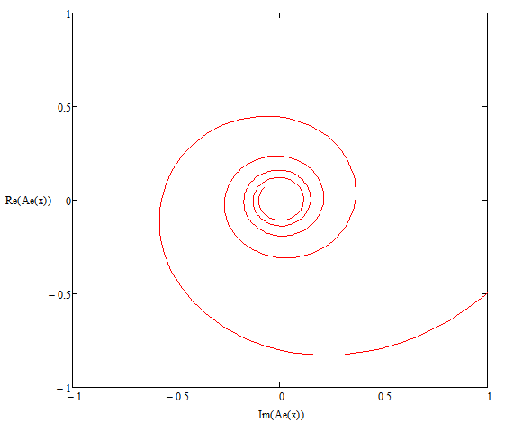Fig.1. Parametric graph of the reduced electron wave function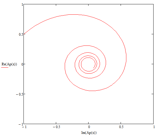

Fig.2. Parametric graph of the reduced proton wave function

Thus, it turns out that the particles create around themselves some all-pervading fields in the form of waves, while the particle itself, as a substance, can no longer be considered in such a context. We will reveal the properties of this field as this theory develops, but at the moment it is clear that it should not be screened. It is also necessary to come up with a name for it, for example, gravel field or G-field. Electric, magnetic and gravitational fields will be only different forms of its manifestation, under certain conditions.

Thus, from a mathematical point of view, the reactive energy \(E_r \) will always have only imaginary values, and the active energy \(E_a \) - only real ones. Their relationship with the total energy is carried out in the classical way - through the Pythagorean theorem: \[E ^ 2 = E_a ^ 2 - E_r ^ 2 \tag {1.5} \]

Based on this, we find the points at which the energy is reactive: \[\left (e ^ {\mathbf {i} (\pi x - \pi / 4)} \right) ^ 2 = \mathbf {i} \tag {1.6} \] hence \[\sin (2 \pi x - \pi / 2) = 1 \] where \[2 \pi x - \pi / 2 = \pi / 2 + 2 \pi n \] where: \(n \) - any integer greater than or equal to zero. From the last expression, we obtain the quantized values of the reactive energy of the electron, in which it can be at \[x = \frac12 + n \quad \tag {1.7} \] which corresponds to the proportions of the quantum harmonic oscillator [1] and reveals its physical meaning. It can even be said that an electron in its normal state, outside the atom and external influencing forces, is such an oscillator. By the way, the corresponding calculation can be carried out for the wave function of the proton.

Despite its apparent simplicity, this conclusion is very important, since in a state of reactive energy, an electron (or proton) does not emit it. This is how one of the problems of electrodynamics is solved, from the theoretical foundations of which it follows that the electron must constantly emit energy.

In the next section, we will show that energy pits also appear in the electron-proton system of the simplest protium atom, however, like any other atom. Interestingly, such holes can exist in all systems, arbitrarily small or large, for example, in such. We will talk about planetary and cosmic scales a little later.

Fig.3. A protium atom with an electron in a Bohr orbit (a), displacement to the center (b) or from the center (c) causes the appearance of an impulse that returns it back to orbit

In such an atom, the interaction between an electron and a proton can be represented as the product of their waves (formulas 1.2 and 1.3): \[p = h R \, A ^ e (x) A ^ p (x) \tag {1.8} \] Immediately, we note that we will measure the result of the interaction using impulse, a physical quantity that characterizes the momentum [7]. The fact is that for a wave, the concept of force is not very suitable because force is directly related to acceleration, and our wave propagates at a constant speed. For the future, you can define the following scheme for yourself: force works well with matter, and momentum works well with a wave. We can even say that the analogue of force for a wave is an impulse, the magnitude of which is directly proportional to the speed, which is what we need.

In the last formula, to obtain impulse values, we established two well-known constants: \(h \) - Planck's constant [8], and \(R \) - Rydberg's constant [9]. Further we will see how their choice was justified. Now we can deduce the final result of the interaction between an electron and a proton in the protium atom: \[p = {h R \over x ^ 2} \exp [\, \mathbf {i} (2 \pi x + \pi / 2)] \tag {1.9} \] Let's analyze the received conclusion. Let us assume that the electron is in an atomic orbit with a Bohr radius: \(r = r_0 \), therefore \(x = 1 \), and its energy is completely reactive (Fig. 4, point 1). Then, according to (1.9), its impulse will also be completely reactive: \(p = p_r \), which from a mathematical point of view means its fully complex value. If, for some reason, the electron begins to leave this orbit, for example, towards the center (Fig.3b), then according to the same formula, a small active component of the momentum \(p_a \) will appear, which will return it to its initial orbit. This component has only valid values.

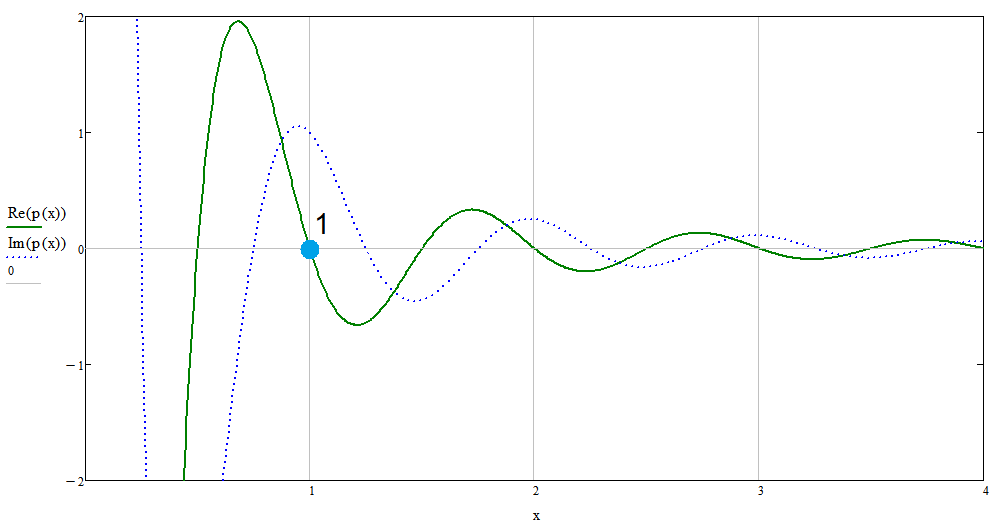Fig.4. Graph of the real (green curve) and imaginary (blue curve) values of the function (1.9), with hR=1

The same can be said for the case when the electron begins to deviate from the center (Fig. 3c), which will cause the appearance of the opposite active component of the pulse, which will return it to the Bohr orbit again. Thus, the physical meaning of the existence of the electron orbit is revealed: in orbit, the electron maintains its optimal energy state, in which all its energy becomes reactive, and in this form is not emitted. But in this case, formula (1.9) assumes its rotation around the proton due to the reactive component. This fact gives an answer to the question of why the electron rotates at all, and what kind of force compels it to do so. It is clear that such orbits are possible when \(x \) takes integer values: \[x = 1, 2, 3, 4, ... \tag {1.10} \] By the way, these orbits are shifted relative to the values of the quantum oscillator (1.6) by \(\pi / 2 \).

Roughly the same can be said about the atom, which until now we have perceived as something incomprehensible and mysterious. But the atom, from our point of view, turns out to be only the optimal form of interaction between an electron and a proton.

The only thing we forgot to say is that the active and reactive components of the impulse, as well as the reactive and active energies (1.5), are interconnected by the classical Pythagorean equation: \[p ^ 2 = p_a ^ 2 - p_r ^ 2 \tag {1.11} \]

In the next section, we will get acquainted with the spin of the waves, which can form different atoms with the same number of particles, we will derive the general form of their interactions, which unites its particular cases in the form of Coulomb's law, the law of universal gravitation and Rydberg's formula.