


2021-12-01
Wave electricity (WEL)
Part 2
Part 2
"… the connecting link between everything
that exists is vibration"
John Keely
that exists is vibration"
John Keely
In the second part, we will combine the laws of Coulomb, Rydberg and universal gravitation into a single law of interactions. In this case, we will not use the concept of mass and charge, but we will apply the wave approach. To do this, we will supplement our model with two more elements, denote four wave functions for the electron and proton, and on their basis we will derive this law.
2.1 Spin and two more particle models
In 1922, an experiment was carried out [1], which determined the presence of a spin in an electron. For our theory, this means that two more elements must be introduced into its model, which differ from the first two (1.2, 1.3) in an oppositely directed imaginary vector. If the parametric graph of an electron and a proton with an initial spin (now we will call it positive or plus) is a spiral twisting clockwise (Fig. 1-2), then an electron and a proton with a negative spin is a counterclockwise spiral. The models of these particles, therefore, will be as follows: \[\overline {A ^ e (x)} = {\overline {N ^ e} \over x} \exp [\, \mathbf {i} (- \pi x / \overline {N ^ e} + \pi / 4)] \tag {2.1} \] \[\overline {A ^ p (x)} = {\overline {N ^ p} \over x} \exp [\, \mathbf {i} (- \pi x / \overline {N ^ p} - 3 \pi / 4)] \tag {2.2} \] The upper line above the parameter will mean that the parameter itself belongs to a group of particles with negative spin. With the resulting model, you can do all the same manipulations as with the previous one, with a positive spin, and get the same results. For example, in the interaction of an electron and a proton with a negative spin, we will also find that the optimal energy orbits are in the wave nodes, and their numbers correspond to positive integers, as in (1.10).
2.2 General law of interactions
The VEL interaction law, in general, looks like this: \[p = {h R \over x ^ 2} \bigg [\Phi_1 ^ e + \overline {\Phi_1 ^ e} + \Phi_1 ^ p + \overline {\Phi_1 ^ p} \bigg] \bigg [\Phi_2 ^ e + \overline {\Phi_2 ^ e} + \Phi_2 ^ p + \overline {\Phi_2 ^ p} \bigg] \tag {2.3} \] Here: \(\Phi_i ^ a \) is the wave function of particles, where \(a \) - indicates that the function belongs to the class of particles (electrons, protons), and \(i \) - - interaction group number. If a line is drawn above the wave function, it means that the spin of this group of particles is negative.
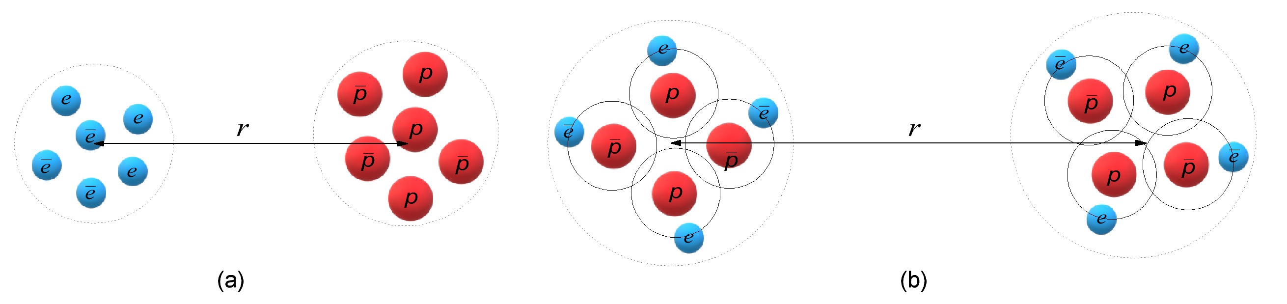 Fig.5. Conventional representation of groups of particles: (a) - electrons in the first group, protons in the second; (b) - in the first group, the particles of the atoms of the first object, and in the second - the second |
By two groups of interaction we mean two sets of particles located at a distance \(x \) from each other, between which we want to know the momentum of interaction. For example, in an atom, the first group can include a set of protons, and the second - a set of electrons (Fig. 5a). In the case of interaction of two atoms, the first group can include a set of particles from the first atom, and the second - from the second. By analogy, if you need to know the interaction between two material objects, then in the first group you can put a set of particles that make up the atoms of the first object, to the second group - from the second object (Fig. 5b).
In the most complete form, the wave functions of an electron and a proton with different spins are presented in the following table:
| \ | Spin + | Spin - |
| Electron | \(\Phi_ {i} ^ e = N_ {i} ^ e \cdot \exp [\, \mathbf {i} (\pi x / N_ { i} ^ e - \pi / 4 + \beta) \,] \) | \(\overline {\Phi_ {i} ^ e} = \overline {N_ {i} ^ e} \cdot \exp [\, \mathbf { i} (- \pi x / \overline {N_ {i} ^ e} + \pi / 4 + \beta) \,] \) |
| Proton | \(\Phi_ {i} ^ p = N_ {i} ^ p \cdot \exp [\, \mathbf {i} (\pi x / N_ { i} ^ p + 3 \pi / 4) \,] \) | \(\overline {\Phi_ {i} ^ p} = \overline {N_ {i} ^ p} \cdot \exp [\, \mathbf { i} (- \pi x / \overline {N_ {i} ^ p} - 3 \pi / 4) \,] \) |
Table 1. Wave functions of an electron and a proton with different spins
where: \(\beta = (\alpha)^8/\pi\sqrt{2} \approx 1.8 \cdot 10 ^ {- 18} \) - the angle of asymmetry between an electron and a proton; \(\alpha\) - fine structure constant. This parameter is responsible for the forces of interaction, which spread even beyond the Debye-Heckel shielding. Also here: \(N_i^g \) - the number of particles in the group, where \(g\) - indicates the group belongs to the class of particles (electrons, protons), and \(i \) - interaction group number. If a line is drawn over the number of particles in a group, it means that the spin of this group of particles is negative.
2.3 Impulse Coulomb Law
One of the special cases of the above general law of interaction is Coulomb's law [2]. We simply remove from the general expression those terms that do not participate in the interaction and obtain a solution for a specific option. Also, we assume that electrons and protons with different spins are involved in the process, and their average statistical value is the same: \[N ^ e = \overline {N ^ e}, \quad N ^ p = \overline {N ^ p} \]
1. For bodies of the same name: \[p ^ {ee} = {h R \over x ^ 2} \bigg [\Phi_1 ^ e + \overline {\Phi_1 ^ e} \bigg] \bigg [\Phi_2 ^ e + \overline {\Phi_2 ^ e} \bigg] \tag {2.4} \] \[p ^ {pp} = {h R \over x ^ 2} \bigg [\Phi_1 ^ p + \overline {\Phi_1 ^ p} \bigg] \bigg [\Phi_2 ^ p + \overline {\Phi_2 ^ p} \bigg] \tag {2.5} \] With the same number of protons and electrons in these formulas, the momenta will be equal to each other: \[p ^ {ee} = p ^ {pp} \] 2. For oppositely charged bodies (Fig. 5a): \[p ^ {ep} = {h R \over x ^ 2} \bigg [\Phi_1 ^ e + \overline {\Phi_1 ^ e} \bigg] \bigg [\Phi_2 ^ p + \overline {\Phi_2 ^ p} \bigg] \tag {2.6} \] With the same number of protons and electrons in the three previous formulas, they also remain equal in magnitude to each other, but the momentum of interaction of oppositely charged bodies turns out to be opposite in sign: \[p ^ {ee} = p ^ {pp} = - p ^ {ep} \] The momentum in these formulas, in principle, can be transformed into force, and then we get Coulomb's law in its purest form.
From this we can draw the following conclusion:
The nature of the Coulomb force lies in the desire of a charged particle to occupy the most favorable energy state. The particle strives to get into the energy wave node.
2.4 Law of gravity in impulse form
Recall that at the moment we are using models of only two types of particles: an electron and a proton, therefore the law of gravitation, in this form, is applicable only for protium atoms. As the species diversity of particles expands, this law will also be supplemented. The form of this law completely coincides with (2.1), since all terms of this expression are used for it (Fig.5b): \[p = {h R \over x ^ 2} \bigg [\Phi_1 ^ e + \overline {\Phi_1 ^ e} + \Phi_1 ^ p + \overline {\Phi_1 ^ p} \bigg] \bigg [\Phi_2 ^ e + \overline {\Phi_2 ^ e} + \Phi_2 ^ p + \overline {\Phi_2 ^ p} \bigg] \tag {2.7} \]
The nature of the gravitational force, as well as the Coulomb force, lies in the desire of the particle to occupy the most favorable energy state. The particle strives to get into the energy wave node.
It is necessary to add here that the same regularity can be traced in all the weapons of nature: living and inanimate. The resulting impulse, as well as in the case of the Coulomb law, can be recalculated into force, and the classical form of the law of gravitation can be obtained. If the number of particles of different types in each group is the same, and \(x / N \ll 1 \) in the exponent of wave functions, then the law of gravitation (2.7) is greatly simplified: \[ p = - 2\beta^2 h R{N_1 N_2 \over x^2}, \quad N_i^e = \overline{N_i^e} = N_i^p = \overline{N_i^p} = N_i \tag{2.8}\] Here: \(N_1, N_2\) - the number of particles in the first and second groups, respectively. The minus sign in front of the expression means that the momentum is directed towards the attraction of these groups, as is customary in physics.
The attentive reader has already noticed that until now we have not used mass and charge, without them we have derived the two most important laws and have determined the orbits of the electron. In traditional physics, without these parameters, it would be simply impossible to do this.
2.5 Rydberg's Law
Let's assign an electron to the first group of particles, and a proton from a protium atom (or any hydrogen-like atom) to the second. Then their interaction will be described as follows: \[p = {h R \over x ^ 2} \Phi_1 ^ e \Phi_2 ^ p \tag {2.9} \] In this formula, \(\beta \) is not taken into account due to its smallness. When all electrons occupy the optimal energy state and the corresponding orbits, then the distance \(x \) between the groups will take only integer values, which follows from formula (1.10) of the previous part. Let's denote these numbers as follows: \[n = x, \quad n = 1,2,3,4, ... \tag {2.10} \] Also, we understand that the number of electrons in an atom will be equal to the number of protons: \[Z = N ^ e = N ^ p \tag {2.11} \] Then the interaction formula becomes: \[p = \mathbf {i} {h R Z ^ 2 \over n ^ 2} \tag {2.12} \] The imaginary unit in front of the right-hand side of the expression shows that the momentum and energy of the particles are in the optimal state. Everything is correct. But what will happen if an electron, being in an excited state in an orbit with \(n = 2 \), goes to a smaller orbit, with \(n = 1 \)? The atom will emit a quantum of Planck energy, equal to \(h \nu \), where \(\nu \) is the frequency of this radiation. Let's deduce the same, but through the impulse and the length of the emitted wave \(\lambda \): \[{h \over \lambda} = p_1 - p_2 = \mathbf {i} h RZ ^ 2 \left ({1 \over n_1 ^ 2} - {1 \over n_2 ^ 2} \right) \tag {2.13} \] where \(n_1 \) and \(n_2 \) - will be the numbers of the final and initial orbits. We already know that being between the optimal orbits, the electron emits energy, which is what happens in our case. Consequently, the reactive energy is converted into active energy of the same amplitude, which means that the imaginary unit in the last expression can be removed. From this we obtain the Rydberg formula [3]: \[{1 \over \lambda} = RZ ^ 2 \left ({1 \over n_1 ^ 2} - {1 \over n_2 ^ 2} \right) \tag {2.14} \] This formula describes well the real spectra of hydrogen-like atoms [4].
2.6 Energy of an electron in orbit
The energy of an electron in orbit can be determined from the formula for the interaction of an electron and a proton (2.12), simply by multiplying it by the speed of light \(c\) \[E_n^e = p c = \mathbf{i} {h R Z^2 c \over n^2} \tag{2.15} \] which fully corresponds in absolute value to the Bohr energy of an electron [5]. The sign of the imaginary unit in front of the expression indicates that this energy is reactive. This advantage of our model immediately gives a physical meaning to this energy. In the standard model, it is made negative, which completely confuses university students :)
In a more general sense, mass is always reactive energy. It becomes active when a particle turns into radiation, for example, into a photon. Then, as we know, the mass disappears.
To be continued...
Materials used
- Wikipedia. Stern-Gerlach experiment.
- Wikipedia. Coulomb law.
- Wikipedia. Rydberg formula.
- Wikipedia. Hydrogen-like atom.
- Wikipedia. Bohr model atom.