

2025-07-30
Projection of the global vector onto our 4D world
Appendix
Why is the speed of light the same in all reference systems
In this appendix to the work on constructing projections of the global vector onto our 4D world,
we will answer questions about why the speed of light is constant in all reference frames, and why it cannot exceed a certain value.
In traditional physics, such questions are usually not considered, but are accepted as a given, and simply postulated.
We will immediately stipulate that all proofs will concern a mathematical point in space moving with a speed of \(v\),
and, in the general case, it can depend on time \(t\):
\[ v = v(t) \tag{1}\]
That is, this proof does not limit other possible objects that can have a superluminal speed.
The answer to the questions posed can be given by our hypothesis about unit space and vector algebra.
First, we will mathematically prove the limitation of the speed of light in any frame of reference, from which the geometric meaning will become clear, and at the end of the work we will present the energetic meaning of such a limitation.
Necessary formulas and geometry
Suppose that the point moves with the velocity \(v_1\) forming the following global vector of velocity,
which we will further abbreviate as -- GVV:
\[ \mathbf{V}_1 = \frac{c}{\gamma_1} \sum \limits_{n=0}^{\infty} \mathbf{j_n} \beta_1^n \tag{2}\]
Here
\[ \beta_1 = {v_1 \over c}, \quad \gamma_1 = {1 \over \sqrt{1 - \beta_1^2}}, \quad n=0,1,2,3,\ldots \tag{3}\]
where:
\(\gamma\) - Lorentz factor,
\(c\) -- the speed of light, \(\mathbf{j_n}\) — unit vectors of coordinates of multidimensional space (in a fixed coordinate system).
Also, in this same coordinate system, the second point moves with a velocity that forms its own GVV:
\[ \mathbf{V}_2 = \frac{c}{\gamma_2} \sum \limits_{n=0}^{\infty} \mathbf{j_n} \beta_2^n \tag{4}\]
\[ \beta_2 = {v_2 \over c}, \quad \gamma_2 = {1 \over \sqrt{1 - \beta_2^2}} \tag{5}\]
This arrangement of vectors is schematically shown in Figure 1a.
Here it is necessary to understand that in fact there are infinitely many coordinates, only the first three of them are reflected.
They are formed by unit vectors: \(\mathbf{j_0}, \mathbf{j_1}, \mathbf{j_2}\)
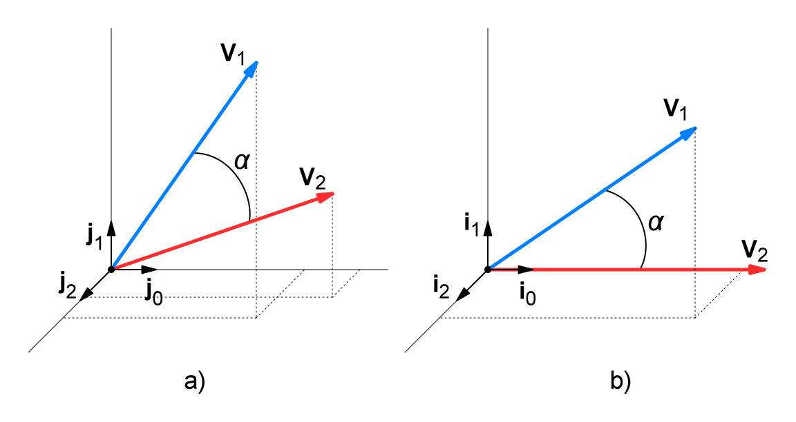
Fig. 1. In the figure: a) - two global velocity vectors and angle α between them, b) - the same vectors in another coordinate system
|
Then, using the rules of vector algebra, we can find the cosine of the angle between these GVV [1]:
\[ \cos(\alpha) = { \mathbf{V}_1 \mathbf{V}_2 \over |\mathbf{V}_1| |\mathbf{V}_2| } \tag{6}\]
where \(|\mathbf{V}|\) is the vector modulus (its length), which, according to the laws of the global vector, is equal to the speed of light:
\[ |\mathbf{V}| = c \]
Then, substituting these modules and scalar multiplying the terms of the two sums from (2) and (4), we get:
\[ \cos(\alpha) = { 1 \over \gamma_1 \gamma_2 (1 - \beta_1 \beta_2) } \tag{7}\]
This angle will remain unchanged in another Cartesian coordinate system.
A convenient coordinate system
It remains to find a more convenient coordinate system for us,
in which the direction of the vector \(\mathbf{V}_2\) would coincide with the direction of the basic unit vector of the new coordinate system (Fig. 1b):
\[ \mathbf{V}_2 \uparrow \mathbf{i_0} \tag{8}\]
We call the first unit vector in the coordinate system by number the basic unit vector, for example \(\mathbf{i_0}\).
Usually it is responsible for the time coordinate.
This new coordinate system is formed by unit vectors: \(\mathbf{i_0}, \mathbf{i_1}, \mathbf{i_2}, \ldots\) in a moving coordinate system.
In it we can also describe the global vector \(\mathbf{V}_1\), but already relative to \(\mathbf{V}_2\):
\[ \mathbf{V} = \frac{c}{\gamma} \sum \limits_{n=0}^{\infty} \mathbf{i_n} \beta^n \tag{9}\]
\[ \beta = {v \over c}, \quad \gamma = {1 \over \sqrt{1 - \beta^2}} \tag{10}\]
Here \(v\) is the velocity of \(v_1\) relative to \(v_2\).
According to the well-known rule of vector algebra, which we have already applied in (6), we find the same cosine of the angle, but between \(\mathbf{i_0}\) and \(\mathbf{V}\):
\[ \cos(\alpha) = { \mathbf{i_0} \mathbf{V} \over |\mathbf{i_0}| |\mathbf{V}| } = { 1 \over \gamma } \tag{11}\]
Let's equate the expressions (7) and (11):
\[ \gamma = \gamma_1 \gamma_2 (1 - \beta_1 \beta_2) \tag{12}\]
Where we find the sum (difference) of the velocities:
\[ \beta = { \beta_2 - \beta_1 \over 1 - \beta_2 \beta_1} \tag{13}\]
But if the velocity \(v_2\) has the opposite direction from \(v_1\), then this expression can be written as follows:
\[ \beta = { \beta_2 + \beta_1 \over 1 + \beta_2 \beta_1} \tag{14}\]
By the way, this formula is derived in STR, but they do it through derivatives, without a clear geometric explanation.
Formula (14) is very important, our proof will be based on it.
Proof #1
With formula (14) it is easy to prove the absoluteness of the speed of light in any frame of reference.
Let's assume that \(v_1\) has reached the speed of light, which means \(\beta_1=1\), then:
\[ \beta = { \beta_2 + 1 \over 1 + \beta_2 \cdot 1} = 1 \tag{15}\]
And this, in turn, means that \(v_2 = c\).
That is, if the speed of the first point is equal to the speed of light relative to a stationary coordinate system, then this speed will be preserved relative to any other moving or stationary point.
The exception is two points moving with the same speed, in the same direction (13).
In this case, obviously, the speed between them will be zero, since, in essence, it will be one point.
And if the speeds are perpendicular?
In a single space, you can get different versions of the speed geometry.
Let's consider another one, when \(\mathbf{V}_1\) and \(\mathbf{V}_2\) are in different coordinate systems, in which the direction unit vectors are perpendicular to each other,
and the only thing that unites them is a common time coordinate (the base unit vector), that is:
\[ \left\{\begin{matrix}
\mathbf{j_n} \cdot \mathbf{i_n} = 1, & \text{if} & n=0
\\
\mathbf{j_n} \cdot \mathbf{i_n} = 0, & \text{if} & n > 0
\end{matrix}\right.
\tag{16}\]
Next, we do the same operations as before (6-12) and first find the cosine of the angle between such vectors from the fixed coordinate system:
\[ \cos(\alpha) = { \mathbf{V}_1 \mathbf{V}_2 \over |\mathbf{V}_1| |\mathbf{V}_2| } = { 1 \over \gamma_1 \gamma_2 } \tag{17}\]
And then we find a new coordinate system in which the base unit vector will coincide with the direction of the base unit vector of the new coordinate system.
From it we find the cosine of the required angle:
\[ \cos(\alpha) = { \mathbf{i_0} \mathbf{V} \over |\mathbf{i_0}| |\mathbf{V}| } = { 1 \over \gamma } \tag{18}\]
After equating (17) and (18), we derive the velocity \(v\), which will show us the velocity \(v_1\) relative to the moving coordinate system \(v_2\):
\[ \beta = \sqrt{\beta_1^2 + \beta_2^2 - \beta_1^2 \beta_2^2 } \tag{19}\]
Unlike formula (14), a square root appears here.
This is understandable, since all the direction vectors (except the base vector) are perpendicular to each other.
Proof #2
Using formula (19), imagine that \(v_1\) has reached the speed of light, which means \(\beta_1=1\), then:
\[ \beta = \sqrt{1 + \beta_2^2 - \beta_2^2 \cdot 1 } = 1 \tag{20}\]
This means that with this formulation of the problem, the speed in the moving frame of reference will be equal to the speed of light and coincide with the speed in the stationary frame.
That is, in this case, the speed of light does not depend on the frame of reference.
Energy
If we introduce the concept of specific energy of a mathematical point as the square of the speed without taking into account the mass,
then it becomes obvious that its speed in our 4D world is only a reflection (projection) of some more global speed.
The global speed of the point itself is always equal in magnitude to the speed of light, which allows it to comply with the same global law of conservation of energy.
We can only change the direction of its movement!
Used materials
- Wikipedia. Dot_product.