In the classical literature [1], the processes in oscillatory circuits (OC) are described quite well, however, for practical application, as a rule, there are not enough specific engineering formulas, with all necessary variants of initial conditions. This paper is dedicated to filling these gaps and can serve as a reminder to the engineer. It will consider two types of circuits - serial and parallel, with several options for the initial conditions in each of them, and in each such variant there are three more cases with possible combinations of the roots of the equation.

For ease of notation, we will use the following form: \[I = I(t), \quad I_{t}^{'} = {\partial I(t) \over \partial t}, \quad I_{tt}^{'' } = {\partial^2 I(t) \over \partial t^2} \] where: \(I(t)\) is the time dependent current and \(t\) is the time.

Here we will consider a sequential OC, and some options for its inclusion in the circuit (Fig. 1). The power supply \(U\) is considered with a constant voltage. Circuits with a variable power supply will be covered in the following chapters.

Then the complete equation of the circuit, according to Figure 1, will be written as follows: \[L\, I_{tt}^{''} + R\, I_{t}^{'} + \frac{1}{C} I = 0, \quad U = const \tag{1.1}\] Here \(L\) is inductance, \(R\) is active resistance, \(C\) is capacitance.

The complete solution to this equation looks like this: \[I = A\, \mathbf{e}^{p_1 t} + B\, \mathbf{e}^{p_2 t} \tag{1.2}\] where \(A, B\) are some constants that will depend on the initial conditions in our chain, and \(p_1, p_2\) are the roots of the characteristic equation, which are found as follows: \[p_{1,2} = -\alpha \pm \sqrt{\alpha^2 - \omega_0^2} \tag{1.3}\] In turn, here: \[\alpha = {R \over 2 L}, \quad \omega_0^2 = {1 \over LC} \tag{1.4}\] Now we can move on to obtaining specific engineering formulas. In this paper, we will not describe in detail how to obtain such formulas; this can easily be done on the basis of the material provided earlier.

Such a variant of the circuit is shown in Figure 1a. We consider the transient process that occurs immediately after the circuit is closed using the \(SW\) switch, the initial conditions of which are defined as follows: \[I(0) = 0, \quad I_t^{'}(0) = {U \over L} \tag{1.5}\] From here, the constants \(A, B\) are found, on the basis of which the formula for the transient process is derived: \[I = {U \mathbf{e}^{-\alpha t} \over 2 \omega L} \left( \mathbf{e}^{\omega t} - \mathbf{e}^{-\omega t} \right) \tag{1.6}\] Here and later in this work: \[\omega = \sqrt{\alpha^2 - \omega_0^2}, \quad \overline\omega = \sqrt{\omega_0^2 - \alpha^2} \quad \tag{1.7}\] The voltage across the resistor \(R\) is found by multiplying it by the current obtained in (1.6): \[U_R = I\,R \tag{1.8}\] The voltage on the inductance \(L\) is sought as a derivative of this current: \[U_L = L\, I_{t}^{'} \tag{1.9}\] Then the voltage on the capacitor \(C\) is found from the sum of the voltages in the circuit: \[U_C = U - U_R - U_L \tag{1.10}\] Based on formula (1.6), we consider three possible combinations of \(\alpha\) and \(\omega_0\) in expression (1.7).

In this case, the transient formula for the current completely repeats expression (1.6): \[I = {U \mathbf{e}^{-\alpha t} \over 2 \omega L} \left( \mathbf{e}^{\omega t} - \mathbf{e}^{-\omega t} \right) \tag{1.11}\] The voltages on the circuit elements will be as follows: \[U_R = U \mathbf{e}^{-\alpha t} {\alpha \over \omega } \left( \mathbf{e}^{\omega t} - \mathbf{e}^{-\omega t} \right) \tag{1.12}\] \[U_L = U \mathbf{e}^{-\alpha t} {(\omega - \alpha) \mathbf{e}^{\omega t} + (\omega + \alpha) \mathbf{e}^{-\omega t} \over 2 \omega} \tag{1.13}\] \[U_C = U \left[1 - {(\omega + \alpha) \mathbf{e}^{\omega t} + (\omega - \alpha) \mathbf{e }^{-\omega t} \over 2 \omega} \mathbf{e}^{-\alpha t} \right] \tag{1.14}\]

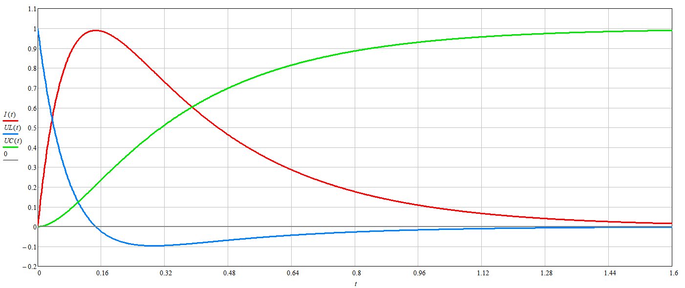
Fig.2. Transient graph 1.2.1: current in the circuit (red curve), voltage on the inductor (blue curve) and voltage on the capacitance (green curve), depending on the time t. Parameters: U=1, L=0.05, ω0=2*π, α=7

The MathCAD routine for this case can be downloaded here.

Here \(p_1 = p_2\). Revealing this uncertainty according to L'Hopital's rule, we get: \[I = {U\, t \over L} \mathbf{e}^{-\alpha t} \tag{1.15}\] The voltages on the circuit elements will be as follows: \[U_R = U \mathbf{e}^{-\alpha t}\, 2 \alpha t \tag{1.16}\] \[U_L = U \mathbf{e}^{-\alpha t}\, (1 - \alpha t) \tag{1.17}\] \[U_C = U - U \mathbf{e}^{-\alpha t}\, (1 + \alpha t) \tag{1.18}\]

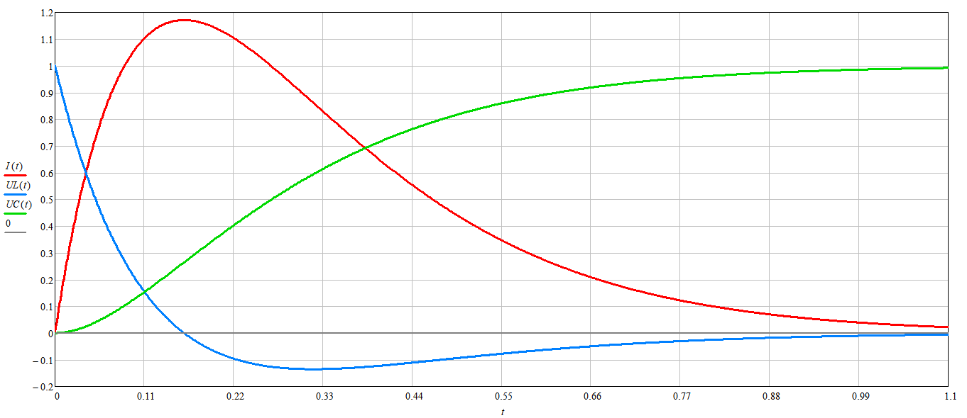
Fig.3. Transient graph 1.2.2: current in the circuit (red curve), voltage on the inductor (blue curve) and voltage on the capacitance (green curve), depending on the time t. Parameters: U=1, L=0.05, ω0=α=2*π

The MathCAD routine for this case can be downloaded here.

In this case, the roots \(p_{1,2}\) are imaginary, and the result of the transient process looks like damped harmonic oscillations: \[I = {U \over \overline\omega L} \mathbf{e}^{-\alpha t} \sin(\overline\omega t) \tag{1.19} \] The voltages on the circuit elements will be as follows: \[U_R = U \mathbf{e}^{-\alpha t}\, {2 \alpha \over \overline\omega} \sin(\overline\omega t) \tag{1.20}\] \[U_L = U \mathbf{e}^{-\alpha t} \left(\cos(\overline\omega t) - {\alpha \over \overline\omega } \sin(\overline\omega t) \right) \tag{1.21}\] \[U_C = U - U \mathbf{e}^{-\alpha t} \left(\cos(\overline\omega t) + {\alpha \over \overline\omega} \sin(\overline\omega t) \right) \tag{1.22}\]

Fig.4. Transient graph 1.2.3: current in the circuit (red curve), voltage on the inductor (blue curve) and voltage on the capacitance (green curve), depending on the time t. Parameters: U=1, L=0.05, ω0=2*π, α=2

The MathCAD routine for this case can be downloaded here.

On the next page, we'll look at a more complex transient where there is an initial current in the coil and an initial voltage across the capacitor (Figure 1b).