Here we consider the transient processes of a series oscillatory circuit (OC), which switches from a constant voltage source \(U_0\) to \(U_1\). Obviously, in this case, some energy is stored in the inductance, and therefore there is an initial value of the current \(I_{0}\) in the circuit, and there is an initial voltage \(U_{C0}\) on the capacitance. The OC inclusion scheme is shown in Figure 1b.

The voltage equation in the circuit does not change and looks exactly the same as the formulas (1.1-1.4) from the previous subsection, but the initial conditions, after closing the key \(SW\), will be different: \[ I(0) = I_{0}, \quad I_t^{'}(0) = {U_1 - R I_0 - U_{C0} \over L} = {U \over L} \tag{2.1}\] The general solution of equation (1.1) in any case will be as follows: \[ I = {\mathbf{e}^{-\alpha t} \over 2 \omega } \left[\left( {U \over L} + (\alpha+\omega) I_0 \right) \mathbf{e}^{\omega t} - \left( {U \over L} + (\alpha-\omega) I_0 \right) \mathbf {e}^{-\omega t} \right] \tag{2.2}\] Here, a kind of initial power source is described by the expression: \[ U = U_1 - R I_0 - U_{C0}, \quad R I_0 = 2\alpha L I_0 \tag{2.3}\] In these and subsequent formulas, it is very important to correctly determine one moment. The direction of the initial current is \(I_0\), which, as we already know, can be both positive and negative (see Fig. 4 - blue curve). In this case, this current flows in the same direction as shown in Figure 1b. If the initial current flows in the opposite direction, then before all \(I_0\), in the formulas of this section, you need to put a minus sign.

Based on formula (2.2), we consider below three possible combinations of \(\alpha\) and \(\omega_0\).

In this case, the transient formula for the current completely repeats expression (2.2): \[ I = {\mathbf{e}^{-\alpha t} \over 2 \omega L} \bigg[\bigg( U + (\alpha+\omega) I_0 L \bigg) \mathbf{e}^{\omega t} - \bigg( U + (\alpha-\omega) I_0 L \bigg) \mathbf{e}^{-\omega t} \bigg] \tag{2.4}\] Here, and further, one should not forget about the nuances with polarity described above. The voltages on the circuit elements, according to formulas (1.8-1.10), will be as follows: \[U_R = {\alpha \over \omega} \bigg[ \bigg( U + (\alpha+\omega) I_0 L \bigg) \mathbf{e}^{\omega t} - \bigg( U + (\alpha-\omega) I_0 L \bigg) \mathbf{e}^{-\omega t} \bigg] \mathbf{e}^ {-\alpha t} \tag{2.5}\] \[U_L = {\alpha^2-\omega^2 \over 2 \omega} \left[ \left( {U \over \alpha-\omega} + I_0 L \right) \mathbf{e}^{-\omega t} - \left( {U \over \alpha+\omega} + I_0 L \right) \mathbf{e}^{\omega t} \right] \mathbf{e}^{-\alpha t} \tag{2.6}\] \[U_C = U_1 - U_R - U_L \tag{2.7}\] Below are the transient graphs for this case.

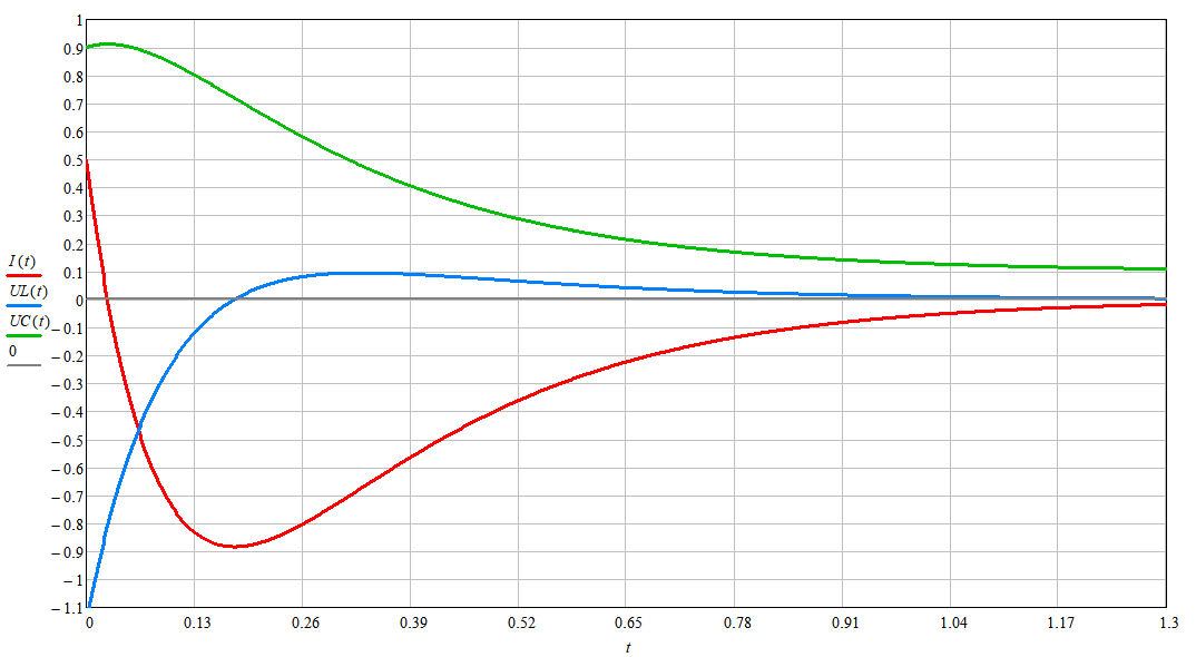
Fig.5. Transient graph 1.3.1: current in the circuit (red curve), voltage on the inductor (blue curve) and voltage on the capacitance (green curve), depending on the time t. Parameters: I0=+0.5, U1=0.1, UC0=0.9, L=0.05, ω0=2*π, α=7

Fig.6. The same graph, but with different initial current parameters: I0=-0.5, U1=0.1, UC0=0.9, L=0.05, ω0 =2*π, α=7

The MathCAD routine for this case can be downloaded here.

Here the roots are equal to each other (1.3): \(p_1 = p_2\). Revealing this uncertainty according to L'Hopital's rule, we get: \[ I = \left[ \left( {U \over L} + \alpha I_0 \right) t + I_0 \right] \mathbf{e}^{-\alpha t} \tag{2.8}\] The voltages on the circuit elements will be as follows: \[U_R = 2 \alpha \left[ \left( U + \alpha I_0 L \right) t + I_0 L \right] \mathbf{e}^{-\alpha t} \tag{2.9}\] \[U_L = \left[ (1 - \alpha t) U - \alpha^2 t\, I_0 L \right] \mathbf{e}^{-\alpha t} \tag{2.10}\] \[U_C = U_1 - \left[ \left( U + \alpha I_0 L \right) (1 + \alpha t) + \alpha I_0 L \right] \mathbf{e} ^{-\alpha t} \tag{2.11}\] Below are the transient graphs for this case.

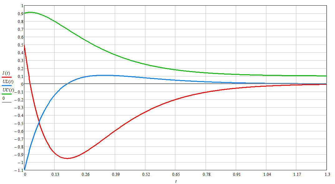
Figure 7. Graph of the transition process 1.3.2. Parameters: I0=+0.5, U1=0.1, UC0=0.9, L=0.05, α=&omega ;0=2*π

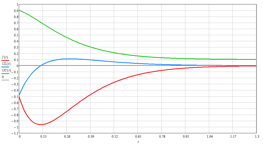
Fig.8. The same graph, but with different initial current parameters: I0=-0.5, U1=0.1, UC0=0.9, L=0.05, .alpha.=.omega;< sub>0=2*π

The MathCAD routine for this case can be downloaded here.

In this case, the roots \(p_{1,2}\) are imaginary (1.3), and the result of the transient process looks like damped harmonic oscillations: \[ I = \bigg[ \bigg( {U \over L} + \alpha I_0 \bigg) {\sin(\overline\omega t) \over \overline\omega} + I_0 \cos(\overline\omega t) \bigg] \mathbf{e}^{-\alpha t} \tag{2.12}\] We only recall that according to (1.7): \[\overline\omega = \sqrt{\omega_0^2 - \alpha_0^2}\] The voltages on the circuit elements will be as follows: \[U_R = 2 \alpha L \bigg[ \bigg( {U \over L} + \alpha I_0 \bigg) {\sin(\overline\omega t) \over \overline\omega} + I_0 \cos(\overline\omega t) \bigg] \mathbf{e}^{-\alpha t} \tag{2.13}\] \[U_L = \left[ U \cos(\overline\omega t) - \bigg( \alpha U + \left[ \overline\omega^2 + \alpha^2 \right] I_0 L \bigg) {\sin(\overline\omega t) \over \overline\omega} \right] \mathbf{e}^{-\alpha t } \tag{2.14}\] \[U_C = U_1 - U_R - U_L \tag{2.15}\] Below are the transient graphs for this case.

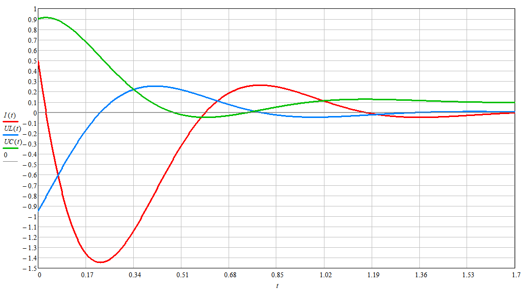
Figure 9. Graph of the transition process 1.3.3. Parameters: I0=+0.5, U1=0.1, UC0=0.9, L=0.05, ω0=2*π, α=3

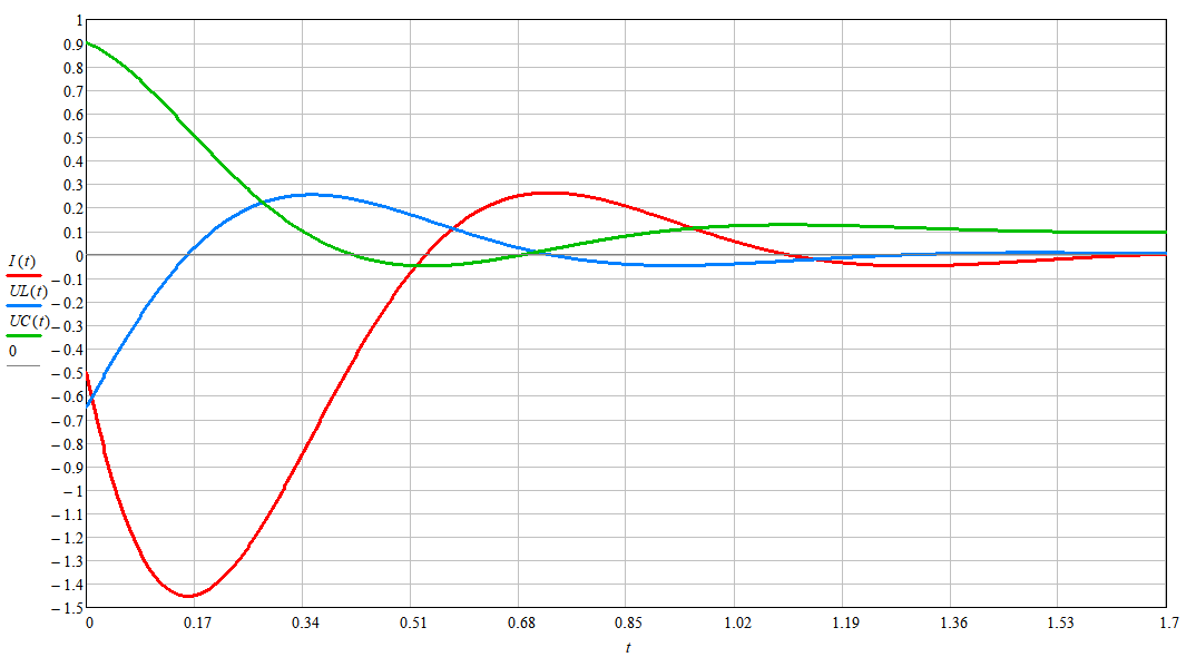
Fig.10. The same graph, but with different initial current parameters: I0=-0.5, U1=0.1, UC0=0.9, L=0.05, ω0 =2*π, α=3

The MathCAD routine for this case can be downloaded here.

This fairly common practical case occurs when the active resistance \(R\) is very small compared to the resistance of the inductance at the frequency of its free oscillations. In other words, when the quality factor of OC is high enough, and is more than 30 units. Recall that the quality factor of a sequential OC is found as follows [1]: \[Q = {\omega_0 L \over R} \tag{2.16}\] Then formulas (2.12-2.15) can be simplified and derived through the quality factor and wave impedance: \[ I = \left[ {U \over Z} \sin(\omega_0 t) + I_0 \cos(\omega_0 t) \right] \mathbf{e}^{-\alpha t} \tag{2.17}\] Recall that the wave impedance of the OC is found as follows: \[Z = \sqrt{L \over C} \tag{2.18}\] and the resonant frequency of the OC is as follows: \[\omega_0 = {1 \over \sqrt{L C}} \tag{2.19}\] Then the voltages on the circuit elements will be as follows: \[U_R = \frac{\mathbf{e}^{-\alpha t}}{Q} \bigg[ U \sin(\omega_0 t) + I_0 Z \cos(\omega_0 t) \bigg] \tag{2.20}\] \[U_L = \bigg[ U \cos(\omega_0 t) - I_0 Z \sin(\omega_0 t) \bigg] \mathbf{e}^{-\alpha t} \tag{2.21}\] \[U_C = U_1 - \bigg[ U \cos(\omega_0 t) - I_0 Z \sin(\omega_0 t) \bigg] \mathbf{e}^{-\alpha t } \tag{2.22}\] Simplified formulas (2.17-2.22) can be used to calculate class D amplifier circuits, and other key stages with inductive-capacitive loads.