

2026-09-09
One-dimensional coordinate of electric interaction:
two experiments with a moving charge
Can an electric sensor distinguish between a charge that is truly accelerating and one passing by at a perfectly constant velocity? And should the same sensor respond to a charge moving in a circle with centripetal acceleration if the distance to the receiver remains constant?
At first glance, the answers would seem to depend on the source's full trajectory and acceleration. However, the two experiments proposed below test a different possibility: that the electric connection between source and receiver singles out only one relative coordinate the distance \(R(t)\)—from the overall geometry. In the first experiment, two completely different motions share the same \(R(t)\) and should produce the same signal. In the second experiment, the charge is constantly accelerating, yet a varying scalar signal appears only when \(R(t)\) begins to change.
The central hypothesis being tested is that the elementary electric connection between a given source and receiver is one-dimensional: its magnitude is determined by a single coordinate, \(R(t)\), while directionality emerges only when this connection is projected into three-dimensional space.
This result takes on special significance in light of the first postulate of "Wave Electricity," which states that in any given physical state, a point possesses only one actual direction of motion. The proposed experiments partially confirm this principle as it applies to electric interaction: regardless of whether the source moves along a straight line or a circle within a two-dimensional plane, the receiver perceives it via the single coordinate \(R(t)\), aligned with the instantaneous "source-to-receiver" connection line. Three-dimensionality manifests in the changing position and orientation of this line, yet the scalar interaction itself remains one-dimensional at any given moment.
This does not yet constitute proof of the fundamental one-dimensionality of the motion; however, it yields an experimentally verifiable consequence of the first postulate. 1. From electric field change to a one-dimensional coordinate
The experimental basis is the sensor discussed in the article “Experiments on Determining Electrodynamic Induction.” As a charged rod moves, the sensor responds primarily to changes in the electric influence. A steady state following the transient process does not produce the same output signal as the approach or withdrawal of the charge.
In the quasistatic approximation, the scalar quantity at the receiver input can be represented as a general function of distance:
\[\tag{1} U(t)=\mathcal F\!\left[R(t)\right]. \] For the electric potential of a point charge, \(U\propto R^{-1}\), whereas for the field strength magnitude, \(E\propto R^{-2}\). To avoid tying the derivation to a specific type of receiver, we introduce a general power law:
\[\tag{2} U(R)=\frac{K}{R^p}, \qquad p=1\, \text{or}\, p=2. \] Then, the rate of change of the input quantity is
\[\tag{3} \frac{dU}{dt} =-pK\frac{\dot R}{R^{p+1}}. \] Formula (3) highlights a fundamental point: the varying signal is determined by the radial velocity \(\dot R\)—that is, by the change in the single coordinate separating the source and the receiver. The source's total spatial velocity does not directly enter this formula. \[\tag{4} \boxed{ \mathbf r_q(t),\, \mathbf r_d(t) \, \longrightarrow\, R(t)=\left|\mathbf r_q(t)-\mathbf r_d(t)\right| \, \longrightarrow\, U(t) \, \longrightarrow\, S(t). } \]
2. Connection to the projectional nature of acceleration
The article "Acceleration as a Projection of Uniform Motion of Higher Splittings" examines two points. One is stationary, while the other moves uniformly in a two-dimensional plane along the trajectory
\[\tag{5} \mathbf r(t)=(ut,d), \qquad \mathbf A_{2D}=0. \] An observer who has access only to the distance between the points obtains the one-dimensional coordinate
\[\tag{6} R(t)=\sqrt{d^2+u^2t^2}. \] Despite the absence of total two-dimensional acceleration, this coordinate has a non-zero second derivative:
\[\tag{7} \ddot R(t)= \frac{u^2d^2}{\left(d^2+u^2t^2\right)^{3/2}}. \] At the moment of closest approach
\[\tag{8} R(0)=d, \qquad \dot R(0)=0, \qquad \ddot R(0)=\frac{u^2}{d}. \] The first experiment transfers this geometry to the electrical dimension. It must determine whether the receiver resolves the full kinematics of the source or perceives only its one-dimensional projection \(R(t)\).
3. General experimental setup
As the source, one can...use an electrified rod; however, for quantitative comparison, a small conductive sphere on an insulating holder is preferable. The sphere is charged before each series of measurements, and its charge or potential is additionally monitored using an electrostatic meter.
The source is moved by a mechanical drive, with its position recorded by an encoder. The receiving unit is based on an electrodynamic induction sensor; however, rather than relying on a simple LED indicator, it is preferable to record the analog output of the amplifier. This allows for the comparison of signal shape, polarity, phase, and amplitude.
If two elongated antennas are used, they must be parallel to each other and aligned with the \(z\)-axis, while all movement should take place within the horizontal \(xy\)-plane. In this configuration, changes in azimuth do not alter their relative orientation, and the distance \(R\) remains the primary geometric parameter governing the coupling.
The experiments are conducted in a low-frequency, quasistatic regime. At low mechanical speeds, any electromagnetic radiation resulting from the charge's acceleration is negligible compared to the near-field electrostatic interaction. Consequently, the study focuses on changes in the scalar electric channel rather than the far-field radiative component.
4. Experiment 1. Different motions with identical R(t)
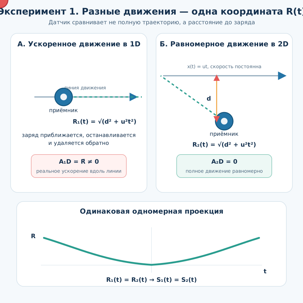 Fig. 1 Actual accelerated motion in one-dimensional geometry and uniform motion in a two-dimensional plane produce the same coordinate \(R(t)\) |
4.1. Longitudinal accelerated motion
The receiver is located at the origin. In the first scenario, the source moves along a straight line passing through the receiver's location but does not reach the receiver itself. The law of motion is specifically defined as follows:
\[\tag{9} \boxed{ R_1(t)=\sqrt{d^2+u^2t^2}. } \] Until the moment \(t=0\), the source approaches; it then stops at a minimum distance \(d\) and begins to move away along the same line. Its velocity and acceleration are
\[\tag{10} \dot R_1(t)= \frac{u^2t}{\sqrt{d^2+u^2t^2}}, \qquad \ddot R_1(t)= \frac{u^2d^2}{\left(d^2+u^2t^2\right)^{3/2}}. \] This is actual accelerated motion along the source-receiver line:
\[\tag{11} A_1(t)=\ddot R_1(t)\ne0. \] 4.2. Uniform passage in a two-dimensional plane
In the second scenario, the source passes the receiver along a straight line located at a distance \(d\). Its position is given by the expression
\[\tag{12} \mathbf r_2(t)=(ut,d). \] The total velocity is constant, so there is no total acceleration:
\[\tag{13} \mathbf v_2=(u,0)=\operatorname{const}, \qquad \boxed{\mathbf A_2=0}. \] However, the distance from the source to the receiver is
\[\tag{14} R_2(t)=\sqrt{d^2+u^2t^2}. \] Consequently, the two series have different total kinematics but the same one-dimensional coordinate:
\[\tag{15} \boxed{ \mathbf A_1\ne\mathbf A_2, \qquad R_1(t)=R_2(t). } \] 5. Prediction for the first experiment
If the electrical coupling is determined by the coordinate \(R\), then in both series
\[\tag{16} U_1(t)=\mathcal F\!\left[R_1(t)\right], \qquad U_2(t)=\mathcal F\!\left[R_2(t)\right]. \] The equality of distances implies the equality of input actions and output signals:
\[\tag{17} \boxed{ R_1(t)=R_2(t) \quad\Longrightarrow\quad U_1(t)=U_2(t), \qquad S_1(t)=S_2(t). } \] Thus, the receiver should not distinguish between a source actually moving with longitudinal acceleration and a source moving uniformly in a two-dimensional plane. To the sensor, both motions appear as a single process: the charge first approaches along the coordinate \(R\), reaches a minimum distance, and then moves away.
The first experiment tests the electrical equivalence of different spatial motions given the same function \(R(t)\). The coincidence of the signals implies that the full trajectory is reduced by the electrical channel to a single relative coordinate.
6. Experiment 2. Rotating charge
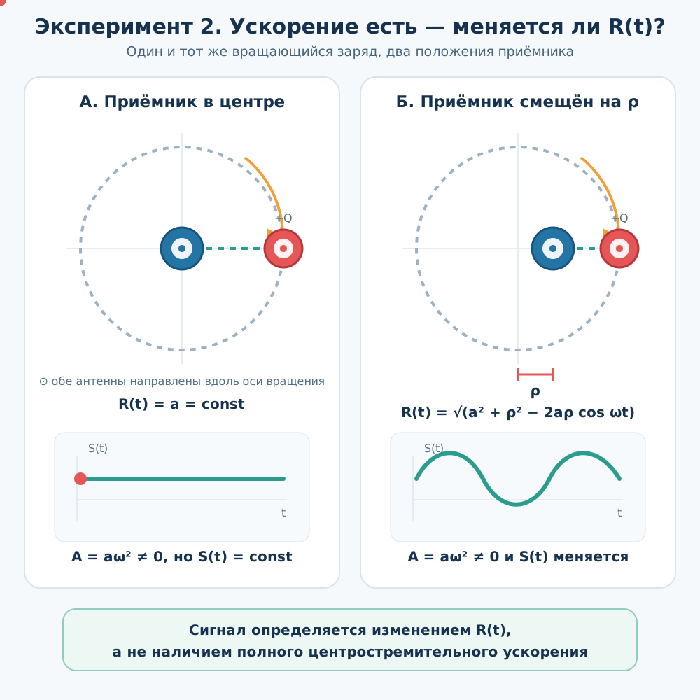 Fig. 2 At the center of rotation, the distance is constant and the scalar signal does not change; after the displacement......the receiver coordinate \(R(t)\) becomes time-varying. |
In the second experiment, a charged source moves uniformly along a circle of radius \(a\):
\[\tag{18} \mathbf r_q(t)= a\bigl(\cos\omega t,\sin\omega t\bigr). \] The magnitude of its velocity is constant, but the direction of the velocity changes continuously:
\[\tag{19} v=a\omega, \qquad \left|\mathbf A\right|=a\omega^2. \] Consequently, the charge possesses the same centripetal acceleration regardless of the receiver's position. The experiment is intended to show whether this acceleration is sufficient to generate a time-varying scalar electric signal.
6.1. Receiver at the center of rotation
First, the receiver is placed exactly at the center of the circle:
\[\tag{20} \mathbf r_d=(0,0). \] The distance from it to the source remains constant regardless of the angle of rotation:
\[\tag{21} R_c(t)=a=\operatorname{const}. \] Therefore, the scalar electric quantity is also constant:
\[\tag{22} U_c(t)=\mathcal F(a)=\operatorname{const}, \qquad \frac{dU_c}{dt}=0. \] The source moves with centripetal acceleration, yet the one-dimensional coordinate of the electric coupling does not change. Therefore, the sensor of variable scalar influence must not produce a periodic signal: \[\tag{23} \boxed{ \left|\mathbf A\right|=a\omega^2\ne0, \qquad \dot R_c=0, \qquad S_c(t)=0. } \]
The first experiment eliminates total acceleration while preserving the same \(R(t)\), and thus preserves the electrical signal. The second experiment, conversely, retains the centripetal acceleration but eliminates the variation of \(R(t)\), thereby eliminating the variable scalar signal. \[\tag{34} \boxed{ \text{The signal is determined by the variation of }R(t), \quad \text{and not by the presence of the source's total acceleration.} } \]
6.2. Why the unknown phase does not create oscillations
The charged antenna and the receiving antenna are oriented along the same axis \(z\), which is perpendicular to the plane of rotation. This setup is axially symmetric. The distance remains constant, the antennas remain parallel at all times, and the line connecting them is always perpendicular to their common axis. Therefore, the mutual capacitance does not depend on the angle:
\[\tag{24} C_{12}(t)=\operatorname{const}, \qquad Q_{\mathrm{ind}}(t)=\operatorname{const}, \qquad U_{\mathrm{pr}}(t)=\operatorname{const}. \] The unknown initial phase of rotation makes no difference here. It could shift the sine wave in time if a fixed component of the field vector within the plane of rotation were being measured. However, the symmetric axial setup does not single out any such direction. The electric field vector may change direction within the plane, while the measured scalar coupling remains constant.
6.3. Receiver offset from the center
Next, the receiver is shifted by a distance \(\rho\) from the center:
\[\tag{25} \mathbf r_d=(\rho,0). \] The distance to the moving charge now becomes a periodic function:
\[\tag{26} \boxed{ R_\rho(t)= \sqrt{a^2+\rho^2-2a\rho\cos\omega t}. } \] It varies within the limits
\[\tag{27} R_{\min}=|a-\rho|, \qquad R_{\max}=a+\rho. \] The radial velocity relative to the receiver is
\[\tag{28} \dot R_\rho(t)= \frac{a\rho\omega\sin\omega t}{R_\rho(t)}. \] Consequently, a variable electric component appears:
\[\tag{29} \frac{dU_\rho}{dt} =-pK \frac{a\rho\omega\sin\omega t} {R_\rho^{p+2}(t)}. \] For a small displacement \(\rho\ll a\), we obtain
\[\tag{30} U_\rho(t) \approx \frac{K}{a^p} \left[ 1+p\frac{\rho}{a}\cos\omega t \right]. \] The amplitude of the variation in the input quantity is linear with respect to \(\rho\), while the amplitude of its derivative is additionally proportional to the rotational frequency:
\[\tag{31} \Delta U_\omega\propto\rho, \qquad S_\omega\propto\rho\omega. \] As the receiver returns to the center, the alternating signal should continuously vanish:
\[\tag{32} \boxed{ \rho\longrightarrow0 \quad\Longrightarrow\quad R_\rho(t)\longrightarrow a, \qquad S_\omega\longrightarrow0. } \] 7. Control measurements
To isolate the desired electric signal from mechanical and electromagnetic interference, the following series of control measurements are performed:
- rotation of the same assembly without a charge;
- measurement with a stationary charged source;
- repetition of experiments with the opposite charge sign;
- changing the direction of rotation;
- varying the speed \(u\) in the first experiment and the frequency \(\omega\) in the second;
- measurement at several values of \(d\) and \(\rho\);
- controlled small displacement of the receiver relative to the center;
- verification of antenna parallelism and shielding of the motor, wires, and power supply unit.
The dependence of the first-harmonic amplitude on the displacement \(\rho\) is particularly important. Near the center, this dependence should be linear and extrapolate to zero at \(\rho=0\). Any non-zero residual value should be compared with the signal from the uncharged rotating assembly.
8. Combined result of the two experiments
The experiments discussed complement each other and allow for the separation of changes in the one-dimensional coordinate \(R(t)\) from the source's full kinematics. In the first experiment, acceleration can be eliminated while maintaining the same \(R(t)\) dependence and the same electrical signal. In the second, conversely, the charge continues to move with centripetal acceleration, yet the signal vanishes if the distance to the receiver remains constant. Let us compare these four states in a single table. | Source motion | Total acceleration | Coordinate R(t) | Variable signal |
|---|---|---|---|
| Longitudinal motion with a turn | Present | Changes | Present |
| Uniform pass-by of the receiver | Absent | Changes in the same way | Same |
| Rotation, receiver at the center | Present | Constant | Absent |
| Rotation, receiver offset | Present | Changes | Present |
9. The one-dimensional nature of the elementary electric connection
The result obtained allows for a simple geometric interpretation. For every pair of electrically interacting objects, there exists a specific line of connection:
\[\tag{35} Q_1 \overset{R}{\longleftrightarrow} Q_2. \] The magnitude of the interaction is formed as a scalar function of a single distance. In the Wave Electricity model specifically in the article “Geometric Origin of Electric Force” the following law was previously proposed:
\[\tag{36} E(R)=E_0\frac{r_e^2}{R^2}, \qquad E_0=\frac{\alpha_{\mathrm{fs}}\hbar c}{e r_e^2}. \] The transition to observable three-dimensional space is accomplished using the unit vector of the connection line:
\[\tag{37} \boxed{ \mathbf E(\mathbf R)=E(R)\mathbf n_R, \qquad \mathbf n_R=\frac{\mathbf R}{R}. } \] Thus, the scalar magnitude of the interaction arises within the one-dimensional coordinate \(R\), while the vector \(\mathbf n_R\) merely defines its direction in the three-dimensional projection. The complete spatial picture of the electric field can be viewed as an aggregate of many such one-dimensional connections.
What is experimentally verified is not the claim that all physical space is literally one-dimensional, but a more precise principle: an elementary scalar electric channel between a source and a receiver is fully described by a single relative coordinate \(R(t)\).
10. Connection to higher-order splittings
In the first experiment, uniform two-dimensional motion is transformed into an accelerated one-dimensional change in distance:
\[\tag{38} \mathbf A_{2D}=0 \quad\longrightarrow\quad \ddot R=\frac{u^2d^2}{R^3}\ne0. \] The hidden transverse coordinate \(d\) compensates for the radial acceleration in the full two-dimensional description. The electric receiver does not recover this coordinate separately and therefore perceives only the accelerated change in \(R\).
In the second experiment, the reverse situation is observed. The full circular motion is accelerated, yet its projection onto the central electric coordinate remains constant:
\[\tag{39} \left|\mathbf A\right|=a\omega^2\ne0, \qquad R=a, \qquad \dot R=0. \] Both experiments demonstrate that the full kinematics of the source and the kinematics of the electric coordinate are not identical. The electric channel performs a geometric reduction:
\[\tag{40} \boxed{ \text{full multidimensional motion} \quad\xrightarrow{\, \Pi_R\, }\quad R(t) \quad\xrightarrow{\, \mathcal F\, }\quad \text{electric signal}. } \] This is a direct experimental analogue of the principle considered in the higher-splitting model: the observed acceleration or lack thereof may be a property of the chosen projection rather than of the entire geometry of the motion.
11. What exactly an experiment can prove
The dependence of pThe dependence of the potential and the electric field magnitude on distance is a known feature of standard electrostatics as well. Therefore, the coincidence of signals in the first experiment and the disappearance of the alternating component at the center of rotation do not, in themselves, constitute unequivocal proof of the physical existence of higher-order splittings.
However, these results establish an important operational property: the chosen scalar electric channel contains no information about the source's full trajectory beyond what is encoded in \(R(t)\). Distinct multidimensional motions become electrically indistinguishable if they share the same \(R(t)\), and accelerated motion produces no alternating signal if \(R\) remains constant.
Within standard electrodynamics, this property is a consequence of the field's radial dependence. Within the framework of Wave Electricity, a stronger interpretation is proposed: the one-dimensional connection is primary, while the three-dimensional field emerges as an aggregate of its directional projections. To distinguish between these interpretations, it will be necessary to identify an additional prediction of the model that is absent from standard electrodynamics.
Conclusion
The first experiment compares actual accelerated motion with uniform motion in a two-dimensional plane. Given the same distance function, they should produce identical electric signals:
\[\tag{41} R_1(t)=R_2(t) \quad\Longrightarrow\quad S_1(t)=S_2(t), \qquad \mathbf A_1\ne\mathbf A_2. \] The second experiment preserves the centripetal acceleration of the charge but alters the position of the receiver. At the center of rotation, \(R\) is constant and there is no variable scalar signal; once the receiver is displaced, \(R(t)\) begins to change, and the signal appears.
\[\tag{42} \boxed{ \begin{gathered} \text{The elementary scalar electric interaction}\\ \text{between the source and the receiver involves a single}\\ \text{directly measurable coordinate, }R.\\ \text{Three-dimensionality manifests itself through the direction }\mathbf n_R\\ \text{and the aggregate of a multitude of such one-dimensional connections.} \end{gathered} } \] Thus, both experiments link the practical measurement of electrodynamic induction to the projective geometry of acceleration. The electric receiver acts as a one-dimensional observer: it perceives not the charge's entire trajectory, but only the change in distance along its own line of connection.